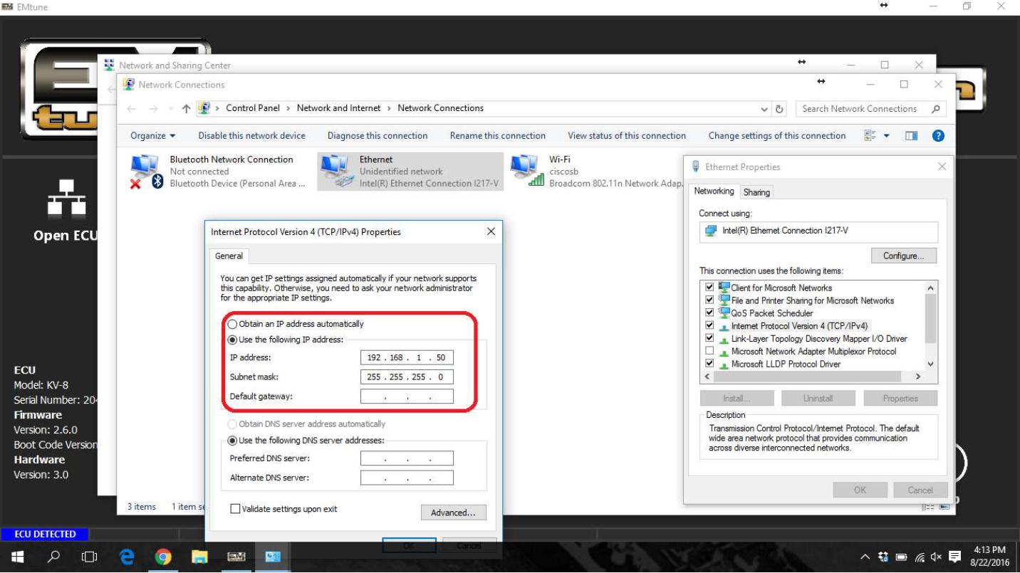
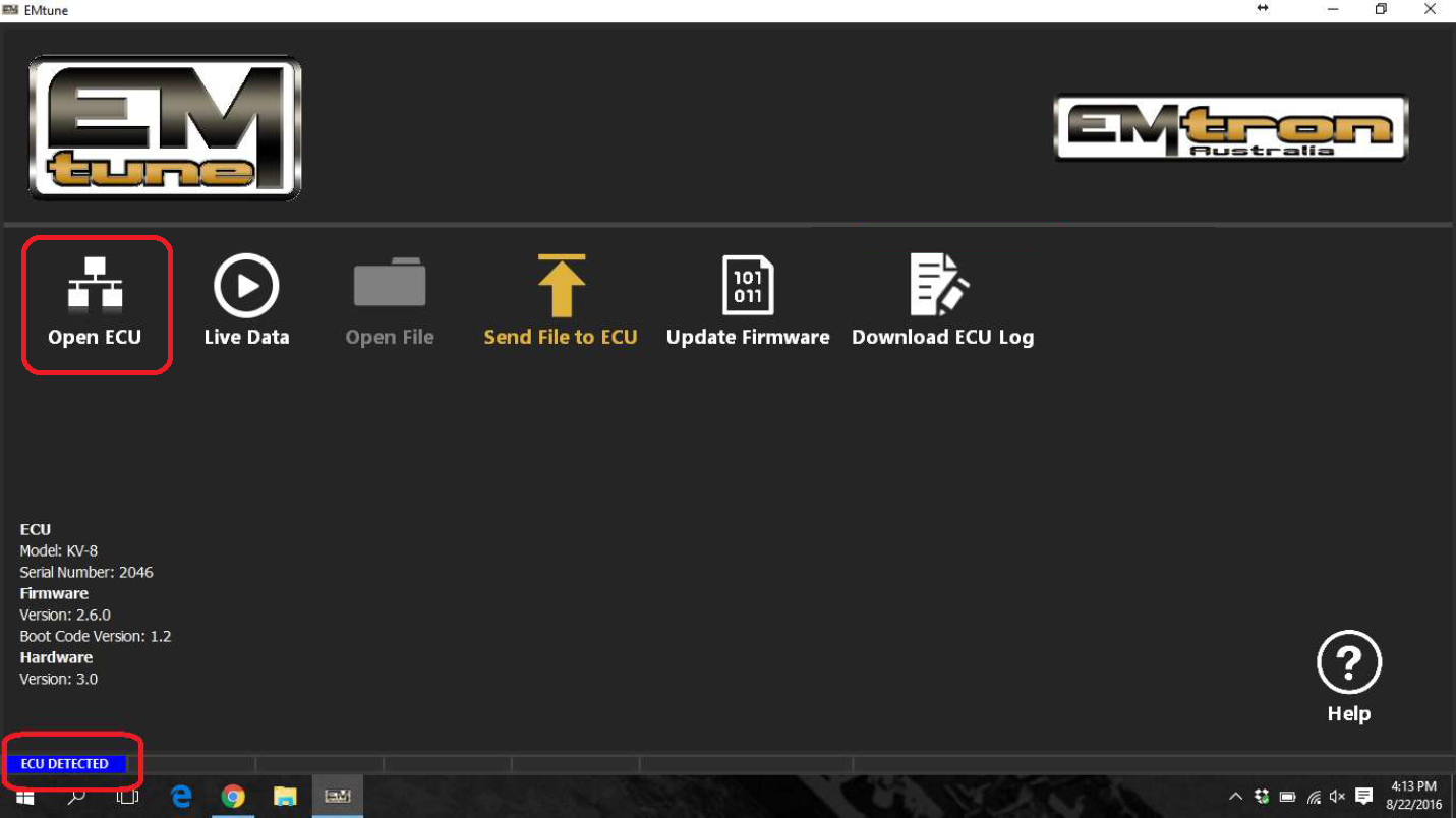
The Emtune software will communicate to the ECU over a static IP address.
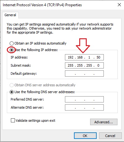
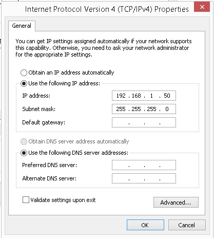
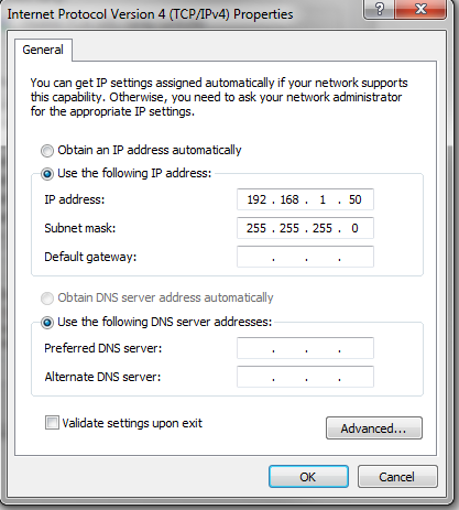
Set your IP and subnet to the following on the Ethernet port you will be using on your PC.
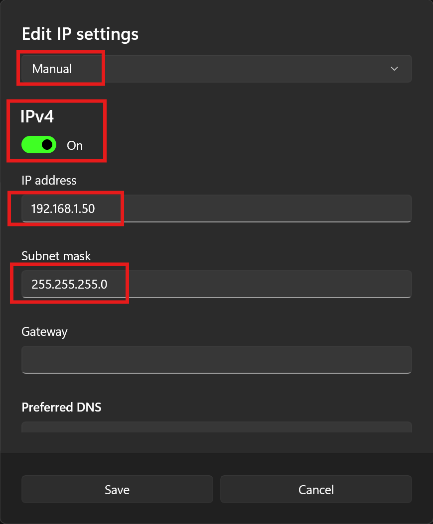
IP: 192.168.1.50
Subnet: 255.255.255.0
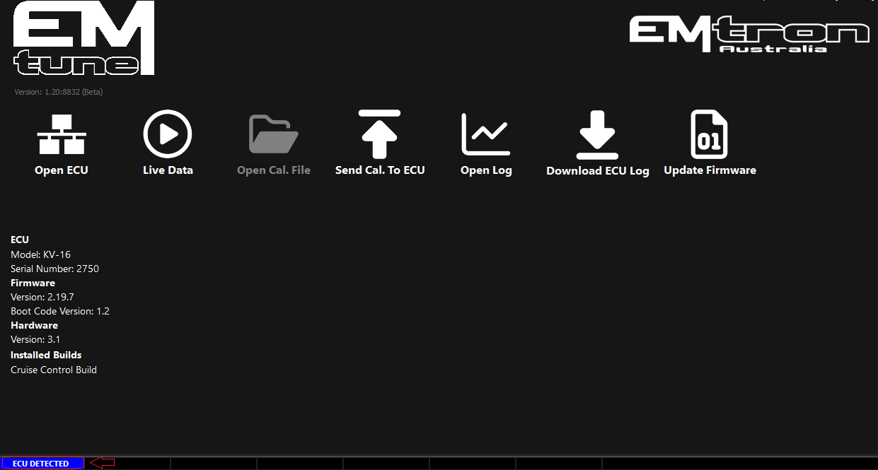
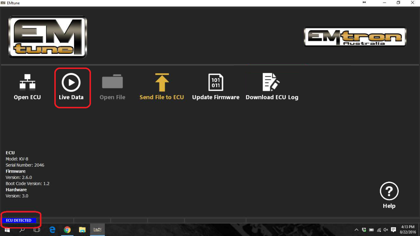
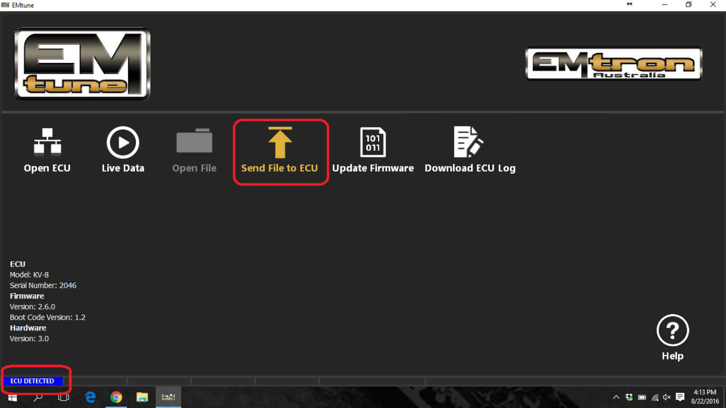
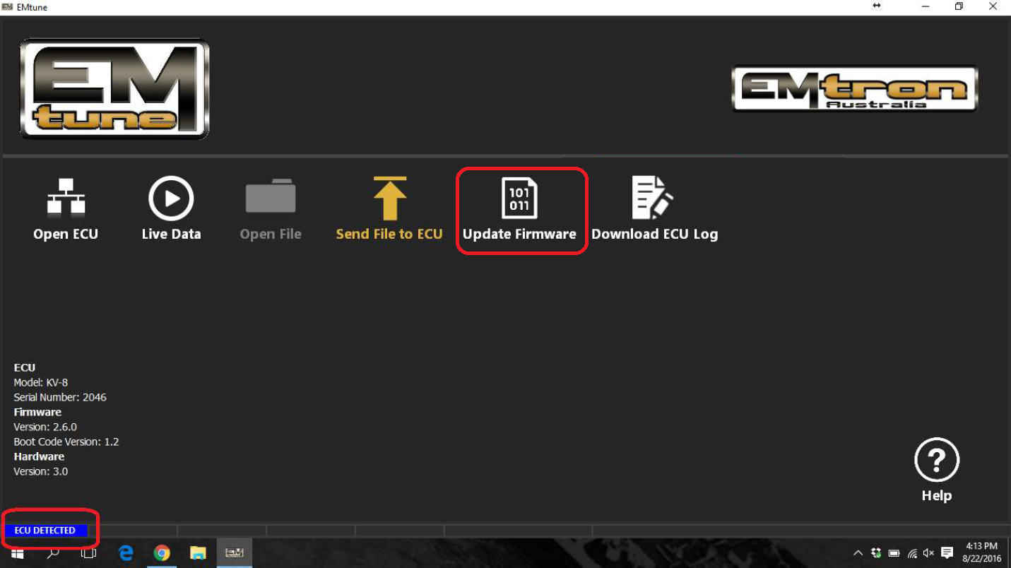
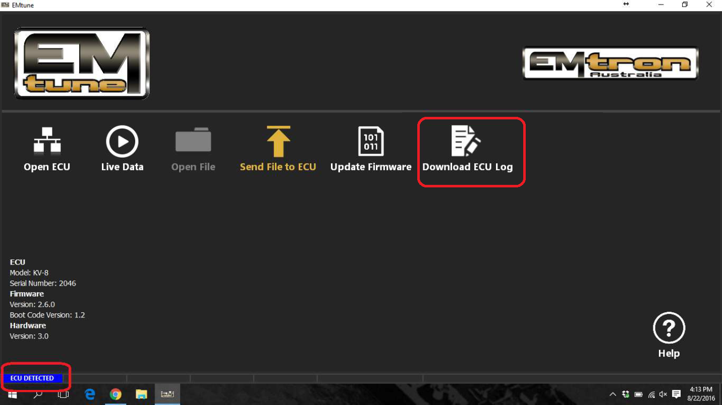
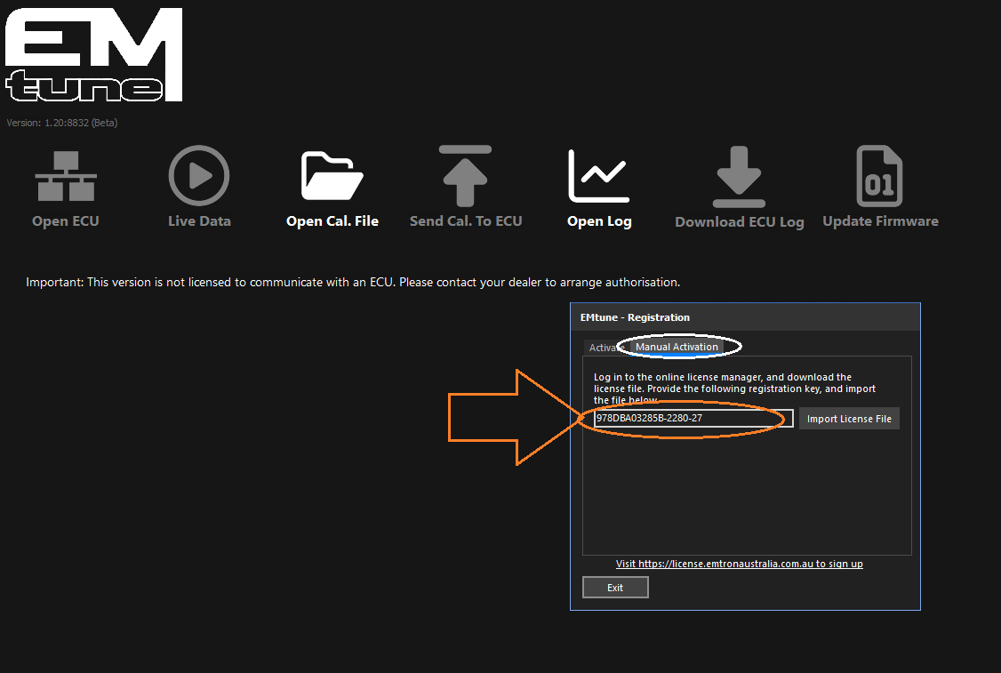
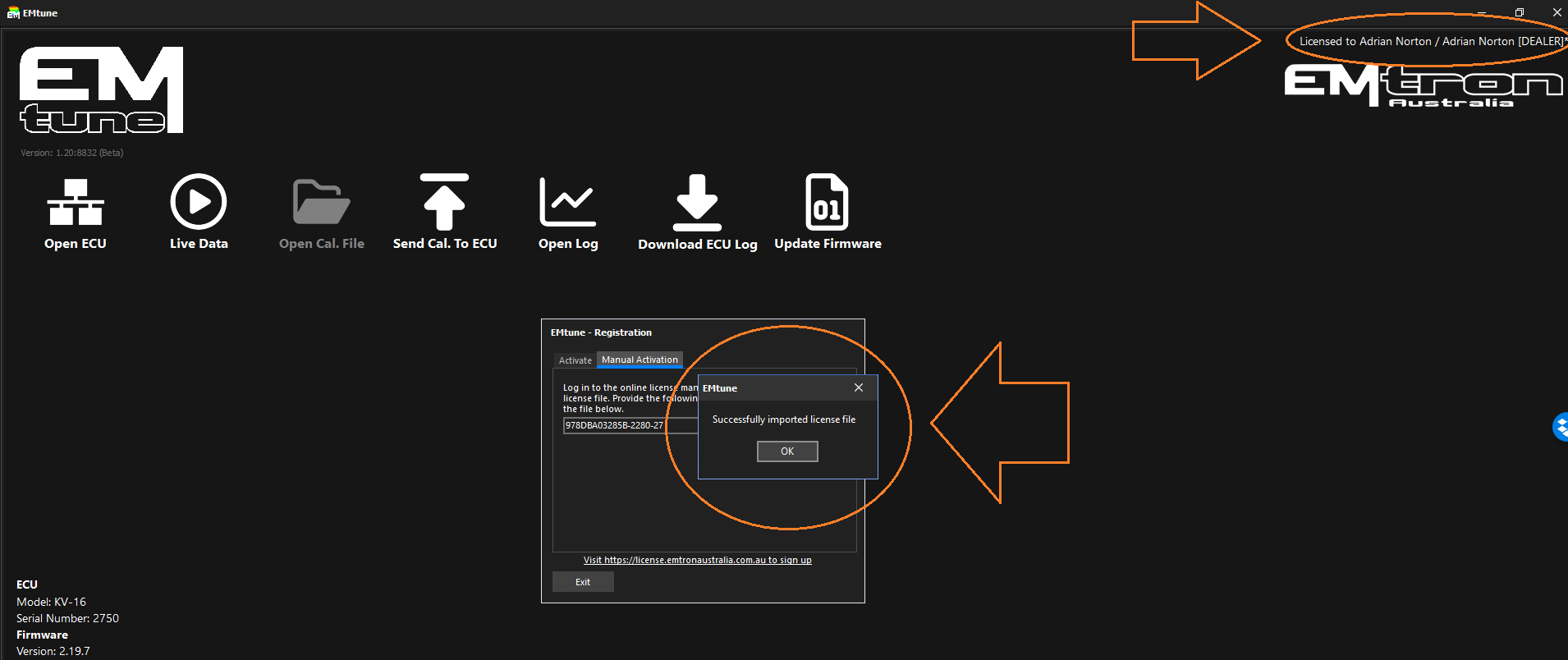
With successful connection, the Emtune Welcome screen will display “ECU DETECTED” in blue in the bottom left corner as can be observed in the background in the above example.
Auto IP Config
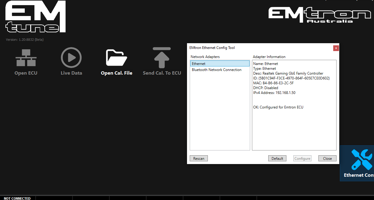
Emtune 1.20.0 and onwards includes a wizard to help configure the ethernet connection (Bottom right of the splash screen)
The wizard may fail to configure the adapter if a previously used adapter was set to the same IP address. Windows can be very finicky about this.
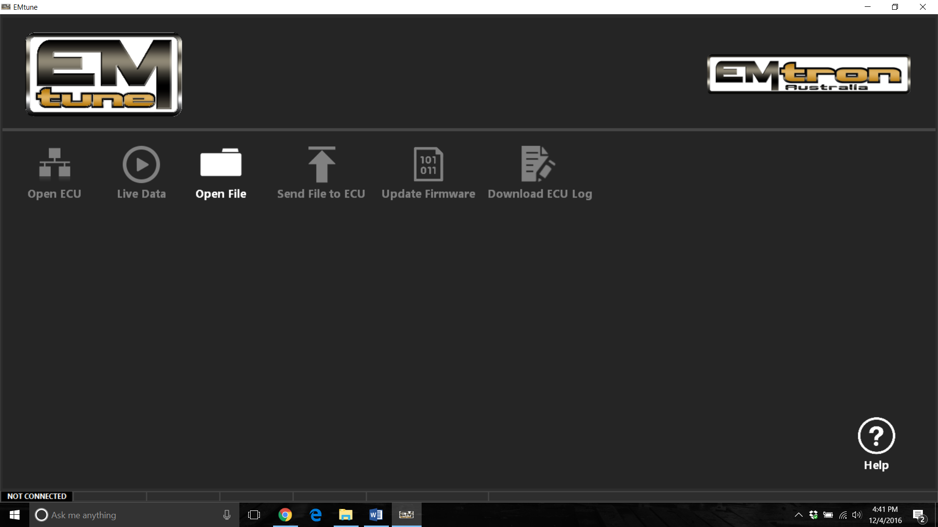
This will be visible when an ECU is no connected / detected.
When the ECU is connected & the IP address correctly configure, the software will acknowledge this in the bottom left corner.
The process to manually configure windows 11+ is as follows:
Manual IP Config
Info on configuring the IP address for different windows version can be found here:
When a correctly configured Ethernet port is in use together with a known good communication cable and you remain unable to establish a connection.
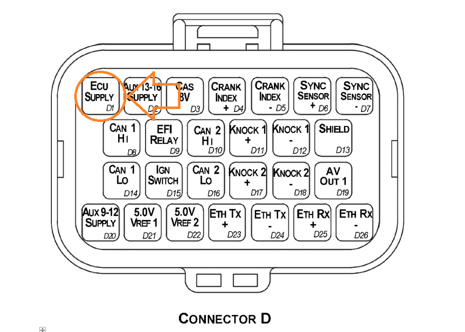
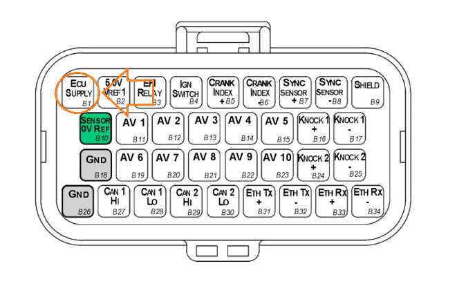
Power supply to the ECU must be verified. That is, the next step is to determine if the ECU is powering up.
Without voltage to the ECU supply pin.
The ECU will fail to power up thereby making communication impossible.
For the KV Series ECU’s this is pin D1
For the SL series ECU’s, this is pin B1
If 12V is not present at D1/B1 with ignition ON, you will need to determine the power supply fault.
Subsections of Ethernet
Windows 11
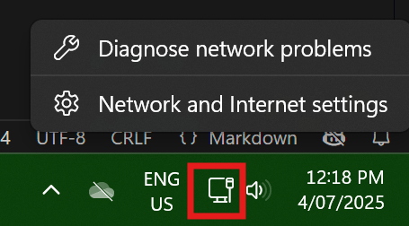
Right click on the Network Connection icon in the system tray. It may appear as a wired connection or a wifi icon.
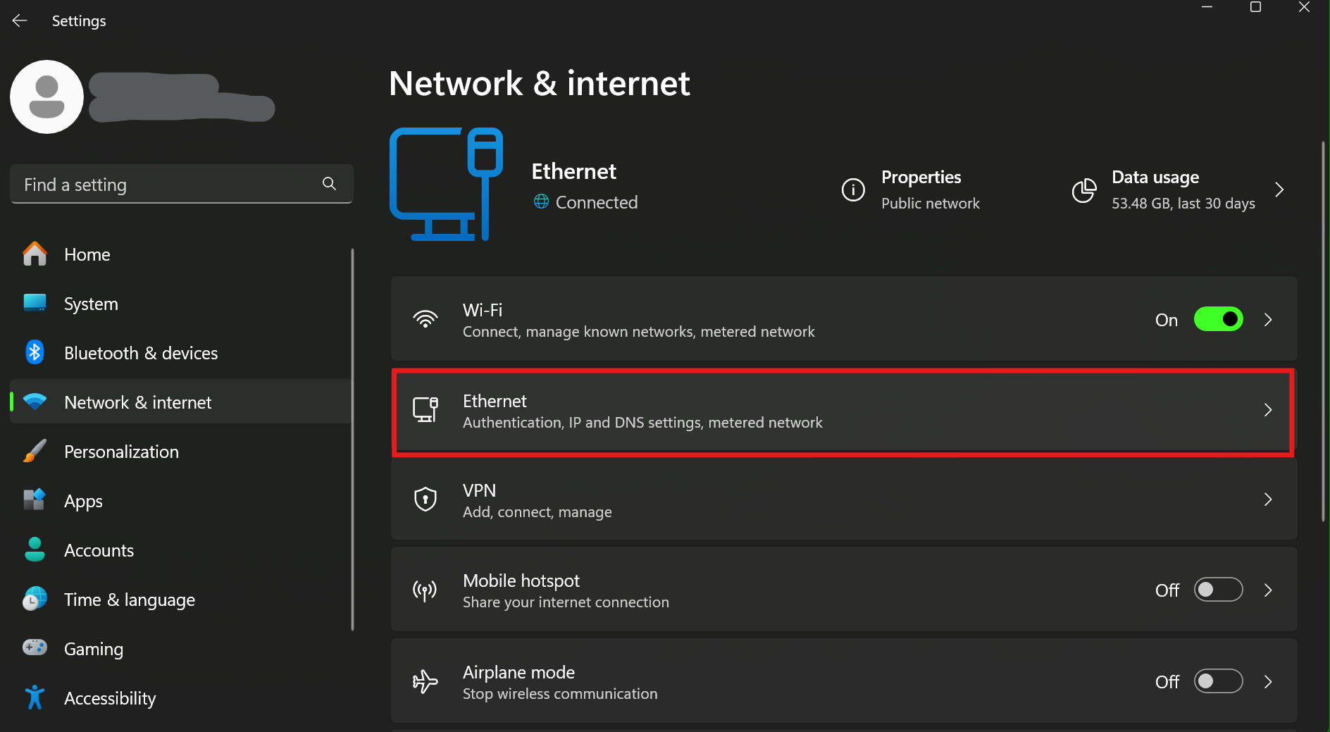
Click on Ethernet
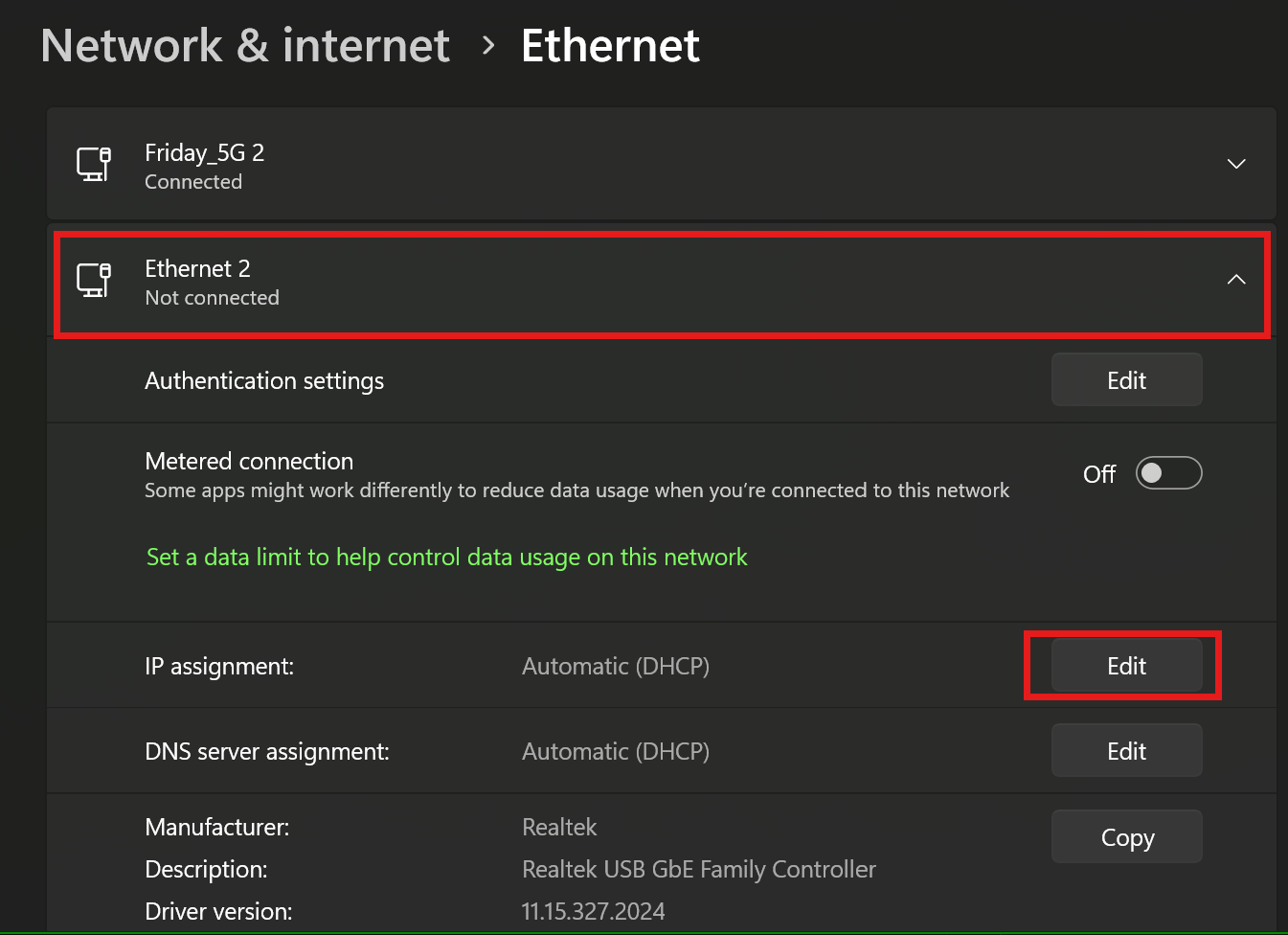
Expand the settings for your ethernet adapter and click on the Edit button for IP Assignment.
Set it to Manual, turn on IPv4, and enter the emtron IP Address and Subnet mask.
Click Save.
Done. Connect the Emtron Ethernet cable.
Windows 10
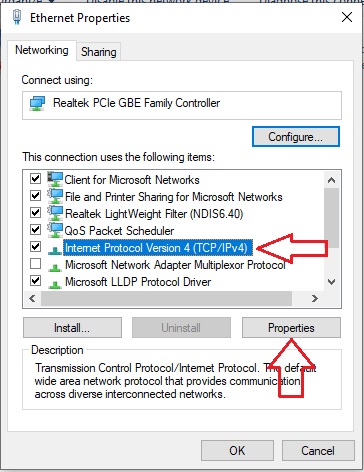
To setup the Ethernet on Windows 10 ready for the ECU connection use the following steps.
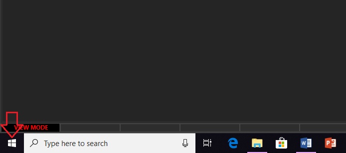
Left Click Windows Icon - Bottom Left corner
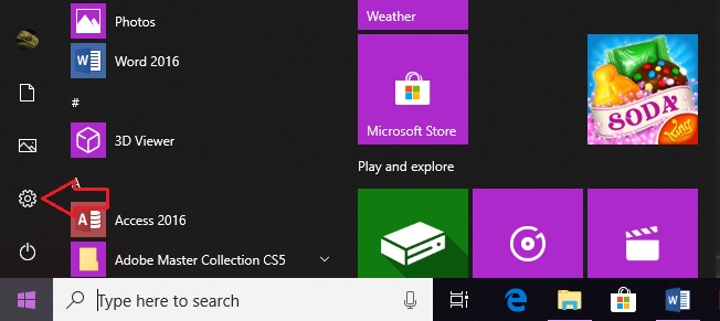
Left Click Settings Icon - 2nd from bottom on Left
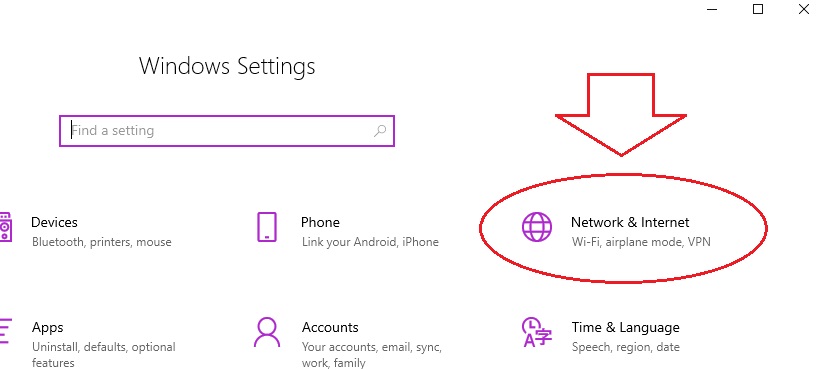
Left Click “Network & Internet” - Top Right
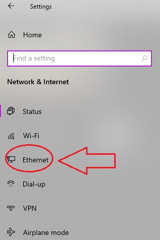
Left Click “Ethernet” - 4th from Top on the Left
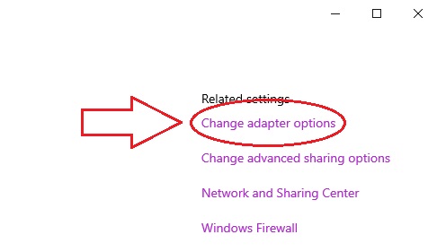
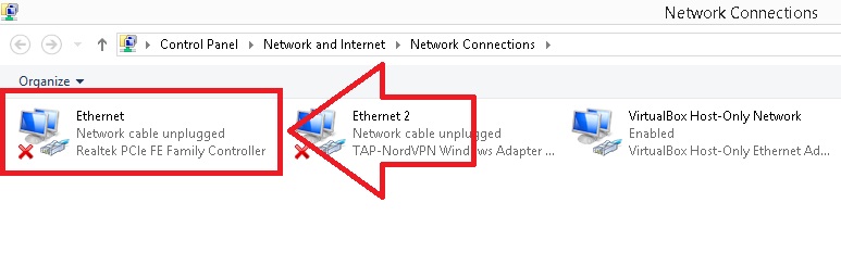
Left Click “Change Adapter Options” - Top Right
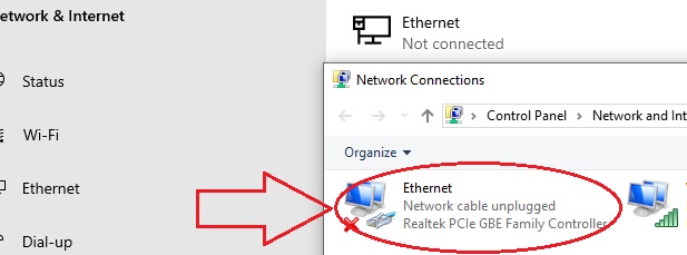
Right Click “Ethernet”
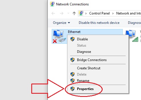
Left Click “Properties”
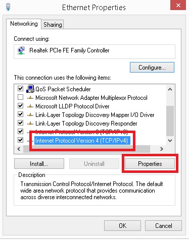
Select “Internet Protocol Version 4 (TCP/IPv4) and Left Click “Properties”
Use the following IP address
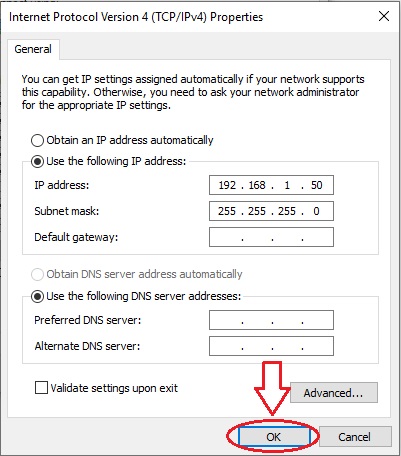
Left Click “OK” and exit, the process is complete
Done. Connect the Emtron Ethernet cable.
Windows 8.1
To setup the Ethernet on Windows 8.1 ready for the ECU connection use the following steps.
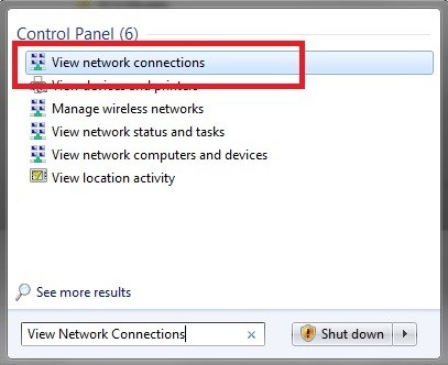
Type “View Network Connections” into the search window, accessed from the start menu. Windows should provide a list of results. Select View Network Connections.
Or alternatively if the search function doesn’t provide this:
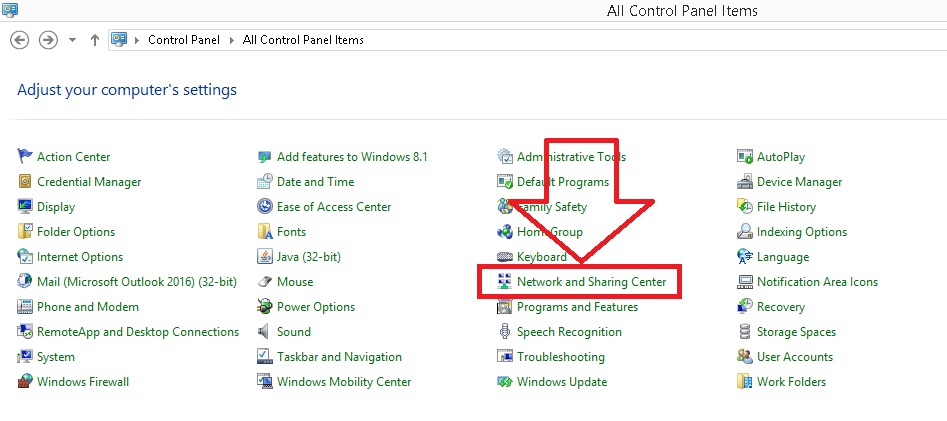
Start > Control Panel > Network and Sharing Center.
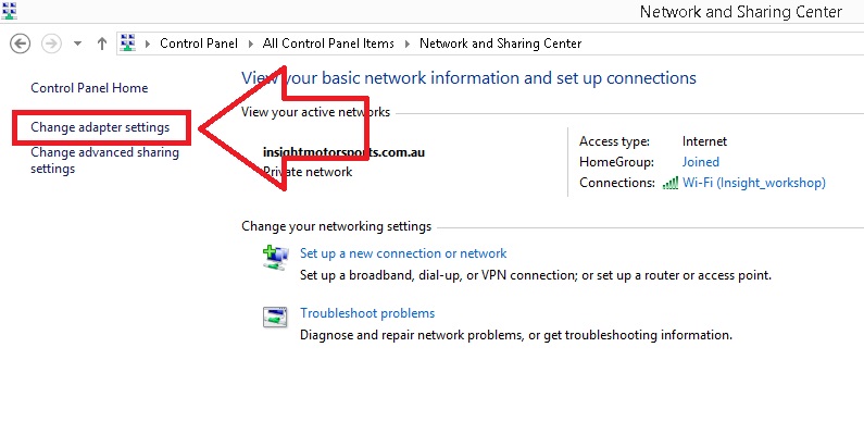
Once in this menu select “Change Adapter Settings”
Once in this menu select “Change Adapter Settings”
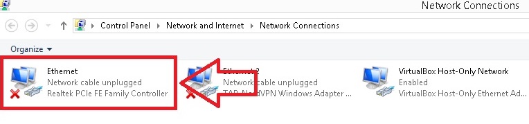
The below menu should be visible. Select “Ethernet”
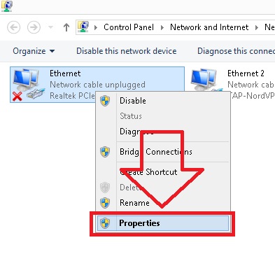
Right click to Access Properties
Select TCP/IPv4 then click Properties
Select “Use the following IP address” and enter in the address 192.168.1.50. The Subnet should automatically default to 255.255.255.0. Click OK.
Done. Connect the Emtron Ethernet cable.
Windows 7
To setup the Ethernet on Windows 7 ready for the ECU connection use the following steps.
Type “View Network Connections” into the search window, accessed from the start menu. Windows should provide a list of results. Select View Network Connections.
or alternatively if the search function doesn’t provide this:
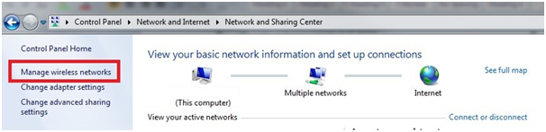
Start > Control Panel > Network and Internet > Network and Sharing Center.
Once in this menu select “Change Adapter Settings”
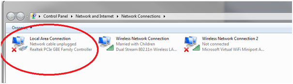
The below menu should be visible. Select “Local Area Connection”
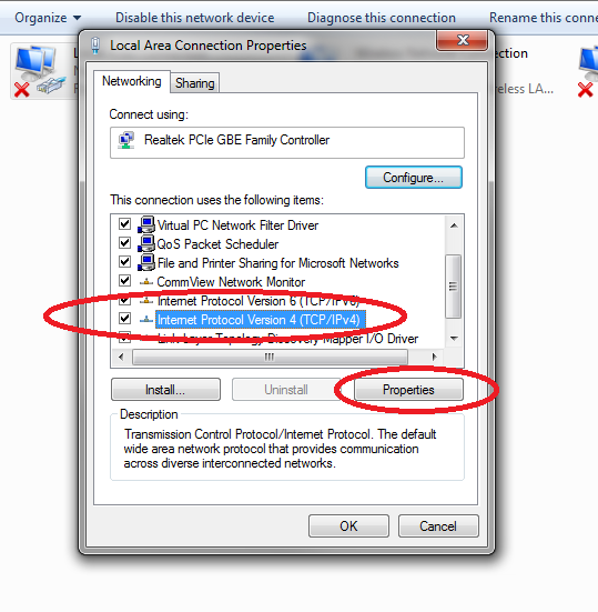
Select TCP/IPv4 then click Properties
Select “Use the following IP address” and enter in the address 192.168.1.50. The Subnet should automatically default to 255.255.255.0. Click OK.
Done. Connect the Emtron Ethernet cable.
Windows XP
Emtune is no longer developed to offer Windows XP compatibility.
Basic Configuration Guide
Software Navigation
From the Welcome Screen, selecting Open File, or Open ECU (ECU Detected is required) the calibration file will be opened.
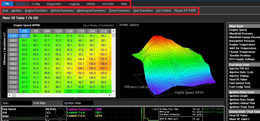
From here, you can navigate through a number of menus, tabs, sub tabs, etc.
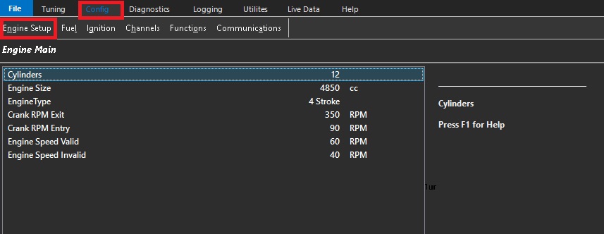
For configuration, clicking the config tab at the top is where to start.
The Emtune software has a very systematical approach to configuration.
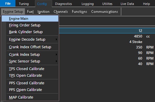
Start on the left side “Engine Setup”, and work your way over from left to right.
Do not skip sections. Following this practice as accurately as possible will ensure tuning process will move smoothly in the future.
Improper entry in any part of the setup could be detrimental to the electronics AND the hardware!
Engine Setup
Setup each tab from top to bottom. See help file for explanation of each individual function, as well as help text in the respective configuration screens.
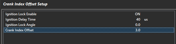
Crank Index Offset Setup
This section synchronizes the engine timing.
**Crank index offset MUST always be checked regardless of trigger pre-configuration.
1)Always check crank index position at ignition lock angle 0.0 (especially when running waste spark).
2) Ignition delay time should be validated at this time and adjusted.
3) As RPM is increased, timing should stay at the ignition lock angle.
If this does not occur - Adjust the ignition delay time until this is achieved.
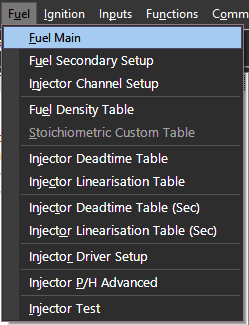
Define all your fuel setting under the Fuel heading.
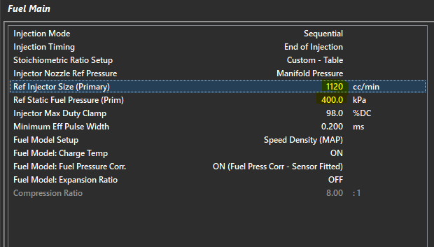
Fuel Flow Rate/Ref Injector Size
The Ref Injector Size flow rate must match the Ref Static Fuel Pressure value
The Ref Static Pressure Value is pressure value that differential/relative fuel pressure at the injector for this injector flow rate value.
** If Fuel Model: Fuel Pressure Corr. Is “On (Fuel Press Corr – Sensor Fitted)”, then this Ref Static Fuel Pressure value is used as the base Fuel Pressure Differential.
The following runtimes will be generated from this information:
Fuel Pressure Diff – This is the effective pressure at the injector
Fuel Pressure Diff Offset – This is the deviation from the differential pressure target (or the reference static pressure entered commonly
Fuel Model Pressure Correction – The percentage of compensation added/subtracted based on differential pressure offset
** If Secondary Injection is used, Fuel Pressure 2 channel MUST be used, and all runtimes above (2) are available and act independently.
These channels can be used all over the ECU calibration, for compensation for deadtime, engine protection, etc.
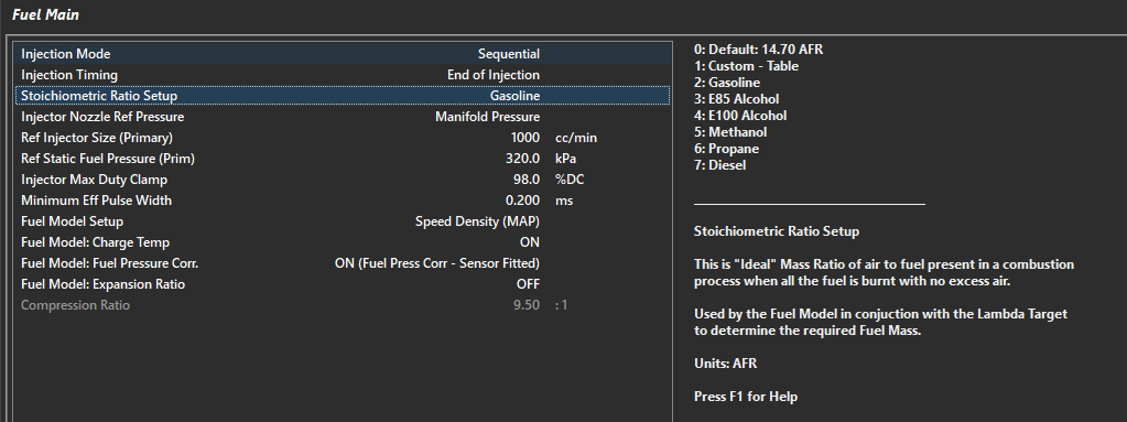
Stoichiometric Ratio Setup
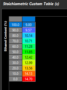
The airflow model will determine air mass flowing through engine a number of ways, then reference the stoich setup to determine how the “Lambda Target” table quantifies the fuel mass needed in the model. There are a number of pre-defined fuel types to choose from, but also a “Custom - Table” selection for pump fuel with ethanol, flex fuel vehicles, etc. See the ECU sample file (Custom - Table), or build your own table if using a odd fuel.
**** Not having the correct Stoich Ratio will bake large error into the entire model and compensations**
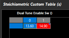
Above is showing how two fuel types can be used with different Stoich values with a “Dual Tune Enable Sw”
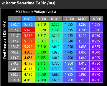
Injector Deadtime and Linearsation
It is very important to have your Injector Size (cc/min) as accurate as possible, as well as the Ref Static Fuel Pressure.
If using any fuel pressure compensation in the model (which you can turn on and off), the Ref Static Pressure is what is used to compensate injection quantity vs effective fuel pressure (differential fuel pressure).
There are 3D table functions for Fuel Density, Custom Stoichiometric (commonly used for flex fuel function), Deadtime, and Linearizion.
**** Injector deadtime accuracy is critical.****
Correct deadtimes ensure the proper amount of pulse width is added to the effective pulse width (as calculated by the fuel model).
Improper time entry usually results in exaggerating VE entries, especially in engine load ranges when the pulse width is small.
It should be taken into consideration that effective fuel pressure affects injector deadtime, so using injectors with good data sheets is the best idea. Most good injectors have a latency multiplier vs fuel pressure, or a complete table available.
These values should be translated and entered into the tables as accurately as possible.
Tuning Tip:
Injector Dead times can be validated using the Emtune Software by using the Wideband Lambda control. If you add 10% to your VE table (@ 3000rpm / 80kpa load for example), you should see a corresponding negative 10% trim applied via the Wideband lambda control. If you don’t, then you know your dead times need some attention.
By utilizing a dead time table available in your Emtune software that is close. The correct dead time for your injector can be quickly arrived at by simply globally moving the table up & down. The voltage slop of the dead times can be further validated by removing the alternator charge and allowing the supply voltage to drop away. Correct dead times allow the engine to operate correctly over a wide range of variable conditions
** Injector Linearization is considered a raw pulse width correction factor to correct the fuel flow at different pulse widths
(generally more sensitive at low pulse widths). These numbers can be positive or negative.
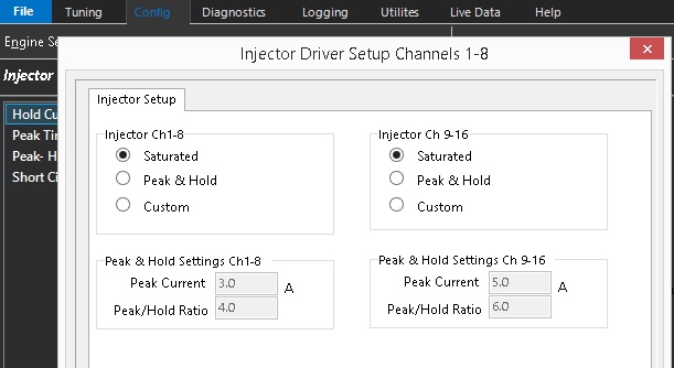
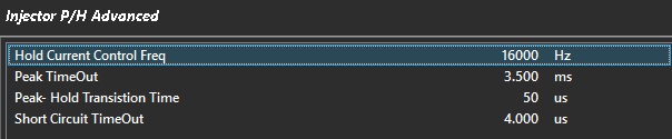
There is a full configuration function for peak and hold injection where you can define the injector type (saturated vs peak and hold), and define opening and hold currents.
The injector test function also allows you to pulse each injector anytime the engine is off.
Ignition
Define all your ignition setting under the Ignition heading.
**Ignition firing edge synchronizes the calculated ignition timing with the physically ignition system itself.
In most cases where the ignition system has ECU controlled dwell (following the dwell table entry), the firing edge will be falling as this is when the coil will inductively transfer spark energy to the spark plug.
Mapped dwell time affects coil charge before this event.
Ignition systems that require the opposite signal (dwell period reversed) generally have a rising firing edge.
Ignition systems that control their own dwell period separately also generally require rising firing edge.
Ignition Timing should be validated with a timing light ALWAYS.
A good test for correct firing edge configuration is to change the dwell time and observe the ignition timing does not change.
Improper set up here can cause false ignition timing, weak spark and even DAMAGE to the ECU or the vehicle Ignition system.
Each cylinder can be assigned two different dwell tables. Each dwell table can be offset by a secondary table as well.
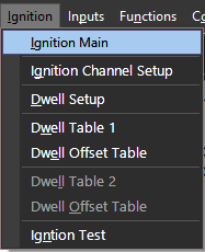
The ignition test function also allows you to pulse each injector anytime the engine is off.
Inputs
This comprehensive setup will specify all Inputs to the Emtron ECU system.
It has a tab structure which has a similar function to the configuration setup.
Input Pins
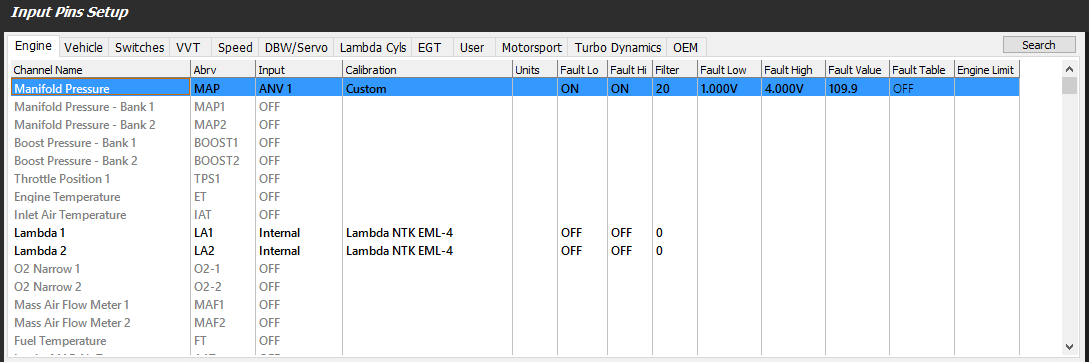
Inputs can be configured using select analog and digital inputs.
The hardware configuration for different ECU types is listed below.
SL Series ECU –
ANV 1-10 12 bit resolution 0-5v analog voltage inputs
ANV 7-10 have switchable pull up to 5v through 1k ohm (temperature)
DI 1-8 0-30khz input frequency range with switchable pull up to 9v through 4.7k ohms
DI 1-8 10 bit resolution 0-20v analog voltage input mode
**KV Series ECU –**
ANV 1-16 12 bit resolution 0-5v analog voltage inputs
ANV 7-12 have switchable pull up to 5v through 1k ohm (temperature)
DI 1-8 0-30khz input frequency range with switchable pull up to 9v through 4.7k ohms
DI 9-14 Standard switch input (low frequency) switchable pull up to 9v
DI 1-8 10 bit resolution 0-20v analog voltage input mode
DI 9-14 Low resolution 0-20v analog voltage input mode
Starting on the left to right and moving through all required and optional inputs and setup.
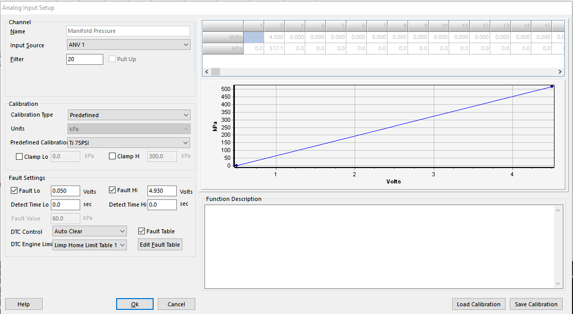
Analog voltage config window:
Sensor input source, filter, calibration, clamp, fault settings, fault value (substitute value), DTC control, and DTC engine limit control are all configured here. There are a number of popular “pre-configured” sensor styles.
If using thermistors, “pull up” must be switched on (only available on ANV 7-10/12).
**Digital inputs can all be pulled up, but they cannot be used for thermistors as the pull up voltage is 9.0V
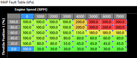
**Major sensors have the ability to enable “fault table” which allows the user to create an active look up table for substitute values.
Example below is for MAP sensor failure, using TP and engine speed to populate active substitute.
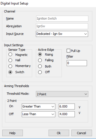
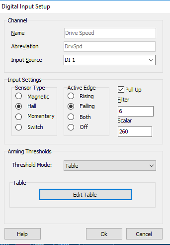
A simple switch configuration for digital input (ignition switch dedicated input):
Input can be configured as a regular toggle switch, magnetic, hall, or momentary switch.
Edge configuration should be appropriately selected based on switch configuration.
Pull up can be used for ground switch inputs (2 point config would be opposite, falling edge trigger).
For high speed inputs, configuration is similar:
High speed inputs (DI 1-8 only) should have “table” as threshold mode, as this will specify the cross over voltage point.
This is similar to “arming thresholds” when configuring triggers
“Scaler” will facilitate the input frequency to unit conversion.
If using KV series internal Lambda sensors, select “Internal” under Input Source
If using CAN bus OEM inputs, select “CANBUS OEM” under Input Source
Custom Runtimes
Efficiency calculation is a runtime commonly used as a load point for fuel tables.
You can select from a number of Emtron calculated runtimes.
Load calculation is a runtime commonly used as a load point for ignition tables and lambda target tables.
You can select from a number of Emtron calculated runtimes.
DI Arming Thresholds
These are the tables generated by high frequency inputs when using the “table” threshold mode.
Lambda Pressure Correction
If using Lambda sensors in situations where exhaust back pressure becomes a factor (Lambda sensor installed before turbocharger or other exhaust restriction), using an exhaust manifold back pressure sensor input allows for correction of the lambda measurement.
Functions
Like Input Pins, this is a comprehensive setup that will specify all outputs to the Emtron ECU system. It has a tab structure which has a similar function to the configuration setup.
Each function that is being used can be enabled here. If there is a required output, then an appropriate output channels can be selected.
An overview of output channel functions from Emtron (see help for more details):
SL Series ECU –
AUX 1-4 Low side
AUX 5-8 Low/High side
AUX 9-10 H-Bridge (One DBW)
Spare fuel and ignition channels can be driven low side
**KV Series ECU –**
AUX 1-8 Low side/high side
AUX 9-12 H-Bridge (Two DBW)
AUX 13-16 Low side/high side
AUX 13-16 H-Bridge (KV12+ - Two DBW)
Spare fuel and ignition channels can be driven low side
**High side drivers and H-Bridge often need control of supply voltage to specified pin locations – see help document
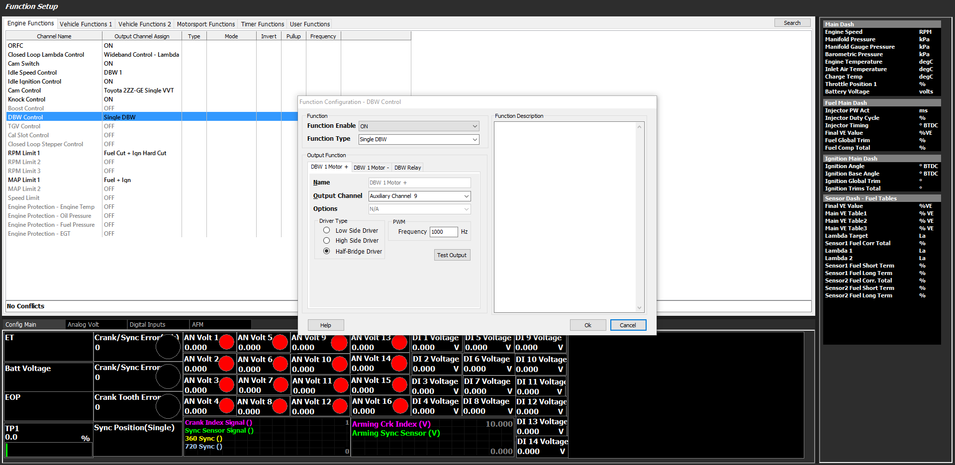
Below is an example of DBW function config.
The mode for DBW is selected, the appropriate output channels, driver type (half bridge), and output frequency.
The same setup is required for any other functions that require outputs.
**See help file for specific functional setup
Communication
This section allows for setup using the Emtron CAN bus channels (2) regarding communication between auxuiliary devices such as dash systems, loggers, EGT devices, as well as Emtron CAN devices (ELC – Emtron Lambda controller).
Besides simple pre-configurations for standard logging sets, advanced setup of this system should be overseen by dealers/Emtron support. Contact your dealer or Emtron support for more assistance.
Continuous Logger
Continuous Logger
When connected to the ECU live, using the “P” key will “Pause” the software completely, and allow the user to navigate back a number of seconds using any line plots on the screen and see exactly where they were in the ECU software.
This mode acts as if they were live tuning the ECU in that very instant.
All hot keys such as “L”, “M”, or any other changes to the calibration are active during this mode, using the paused channel information available at that time.
ECU Password Protection
ECU Password Protection
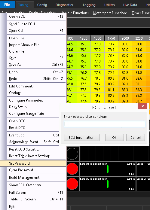
All Emtron ECU’s have the ability to be locked to prevent access from others
This function is access through the main file menu
The Password Protected File cannot be viewed or recovered unless the correct password is known.
Removing Password Protection
If the password is known, this can be done through the main file menu using the Clear Password function
If the password is not know and cannot be retrieved and the ECU must be accessed; the following steps apply.
Sending a Calibration (Cal) File to a Password Protected (Locked) ECU
Any Cal file can be sent to a locked ECU.
Sending a file will load the new Cal file settings into the ECU.
Sending an alternative file will result in the removal of all current ECU settings including the existing password
(when enabled).
There are 2 possible conditions:
The Cal file being sent is Locked. The Cal file will be sent immediately to the ECU overwriting the current ECU file. After the download is complete and the ECU powered cycled the ECU will be locked and you will need the correct password to open the ECU.
The Cal file being sent is Unlocked. The Cal file will be sent immediately to the ECU overwriting the current ECU file. After the download is complete and the ECU powered cycled the ECU will be unlocked.
ECU Runtimes
ECU Runtimes
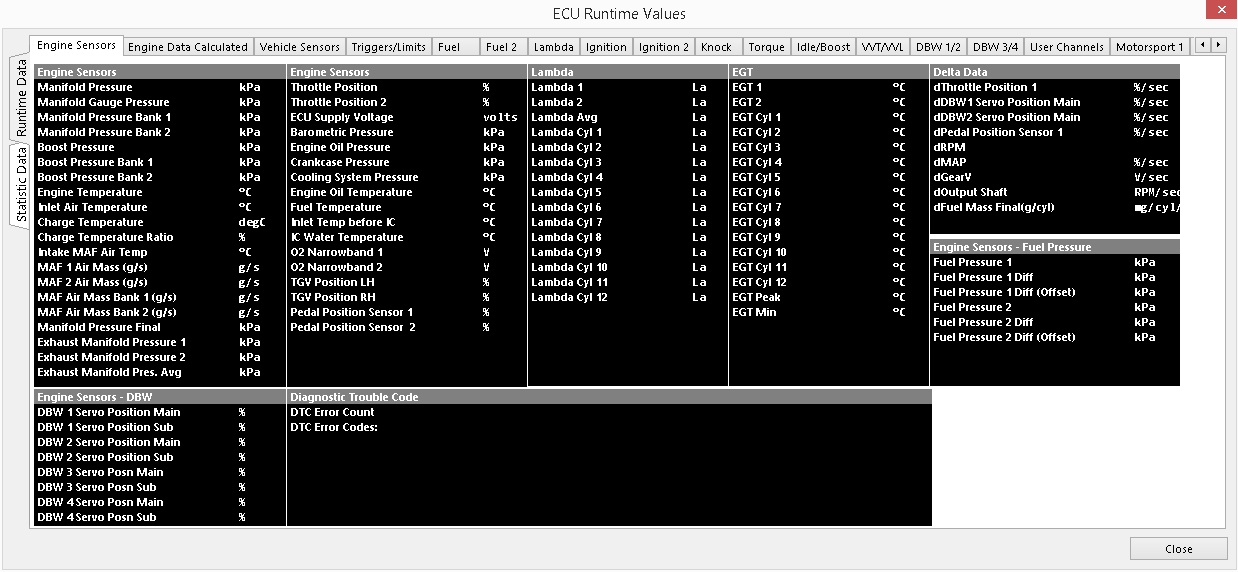
The ECU Runtimes can be accessed by pressed the F3 key or selecting the following menu item:
Emtune Dash Panel Configuration
Emtune allows the user to customize the dash panel screens to suit their needs accordingly.
When opening Emtune for the first time (also when updating software versions), Emtune will ask if you want to overwrite the existing layouts for both the dash panels and the logger with new default configurations. Select accordingly.
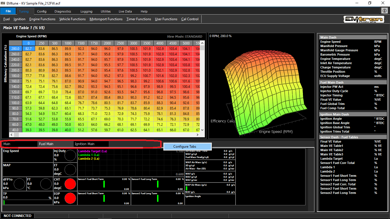
Right Click the Tab section to select Configure Tabs to edit tabs and visibility:
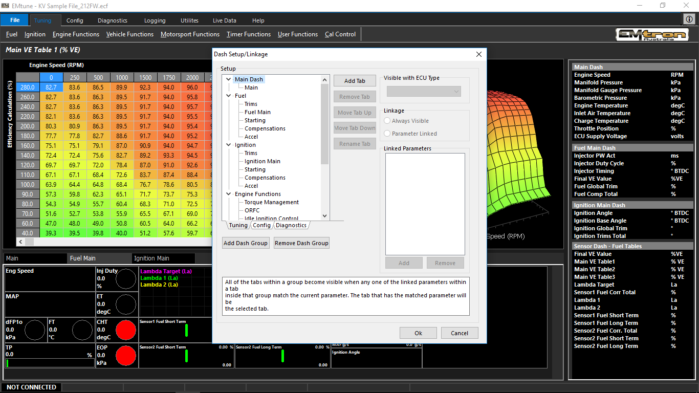
The dash panels are organized by Dash Groups located in the Setup section
** If a function in the software does not have linked view (see below), Main Dash, Main panel will be displayed.
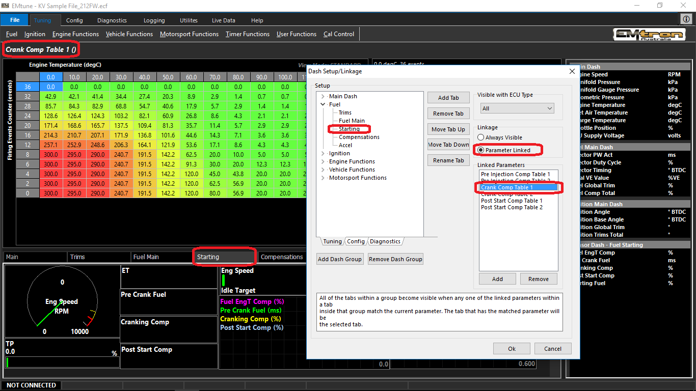
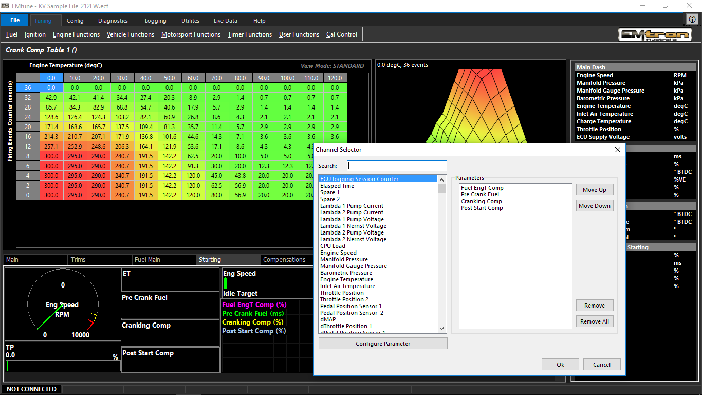
In each dash group, tabs can be created which then can point a software function to that panel. To connect the software to that particular display panel, select Parameter Linked, then add the table to the list. The ECU will then always select that display tab when in the table being viewed (in the case below, Starting, Cranking Comp Table 1).
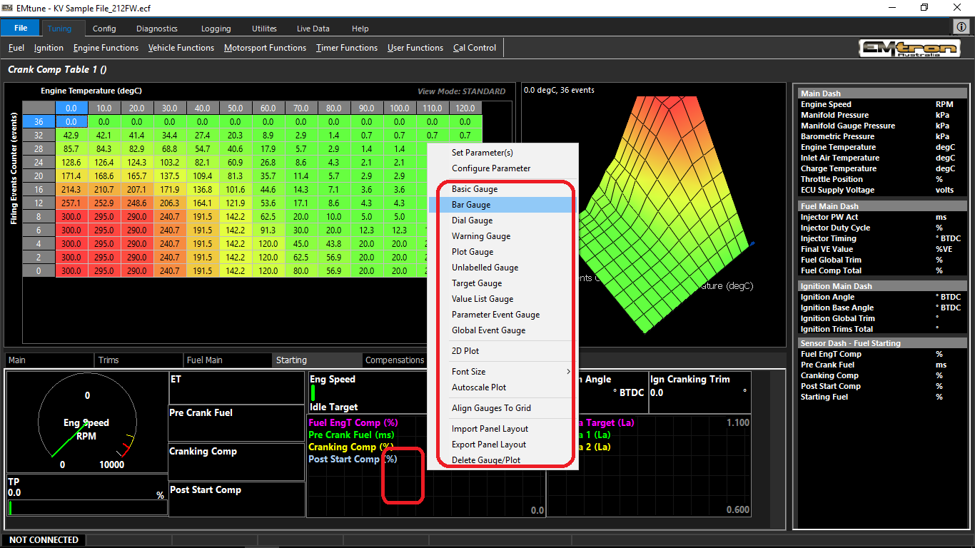
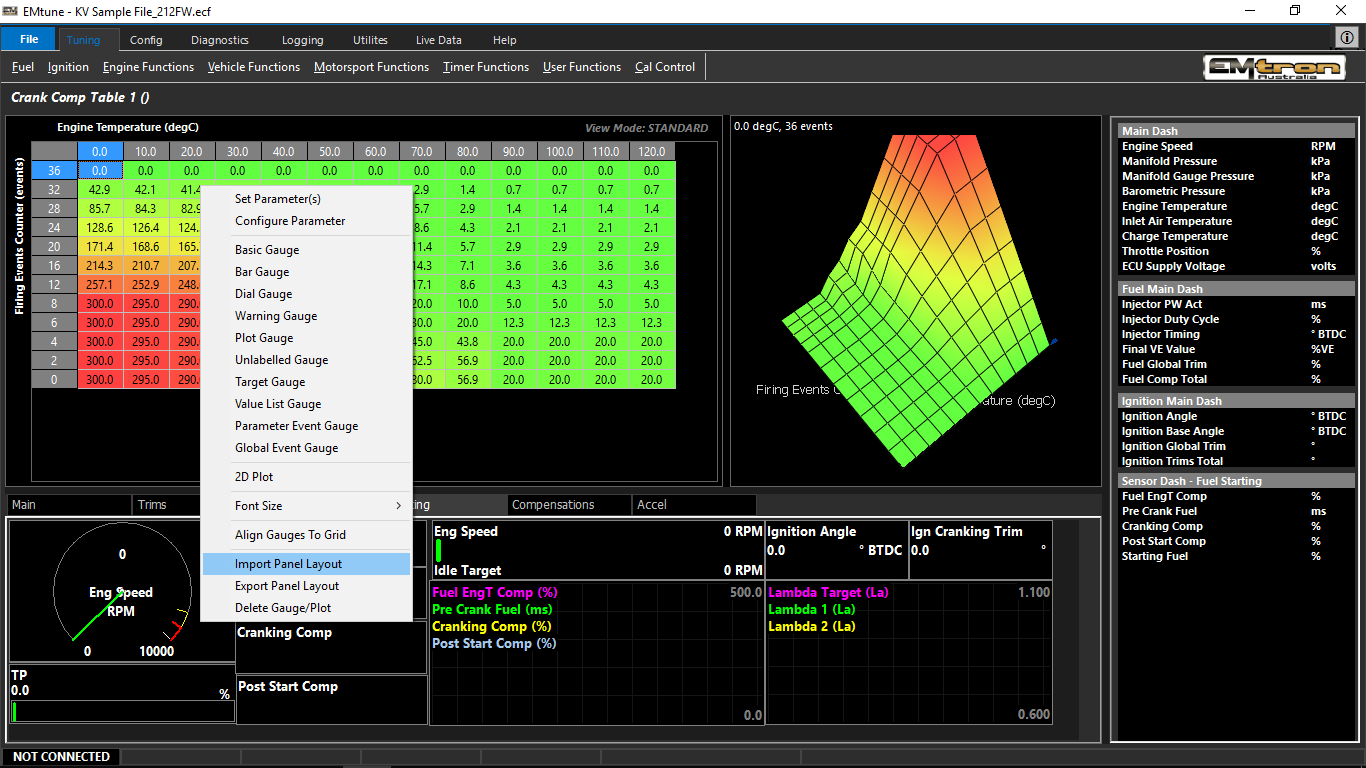
Right click the panel to change, edit, add, replace gauges in the active panel.
Set parameter allows you to define what runtime you want to display. In the case where the display gauge/plot can display more than one runtime, you can add multiple to the list
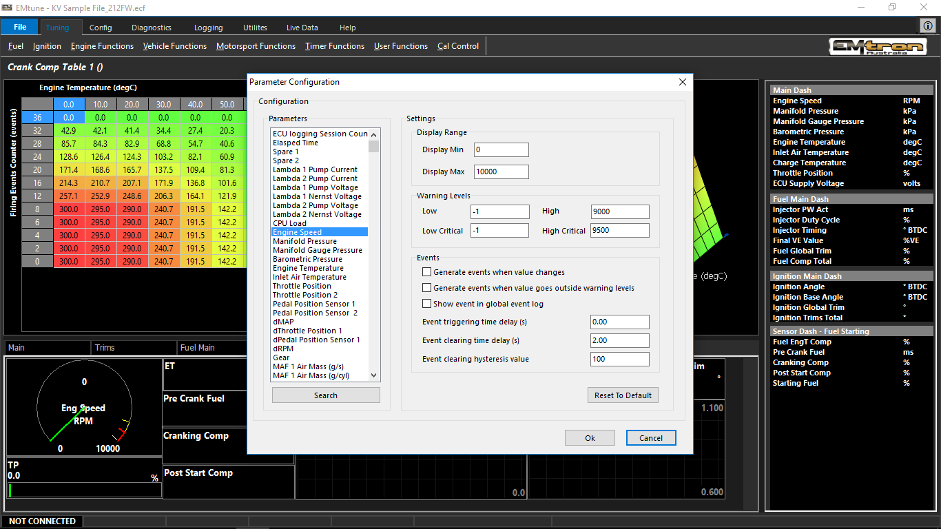
Configure parameter allows you to define the min/max scales for gauges, bar graphs, warning gauges, etc.
Each panel can individually be imported/exported at the bottom of the list when right clicking the panel
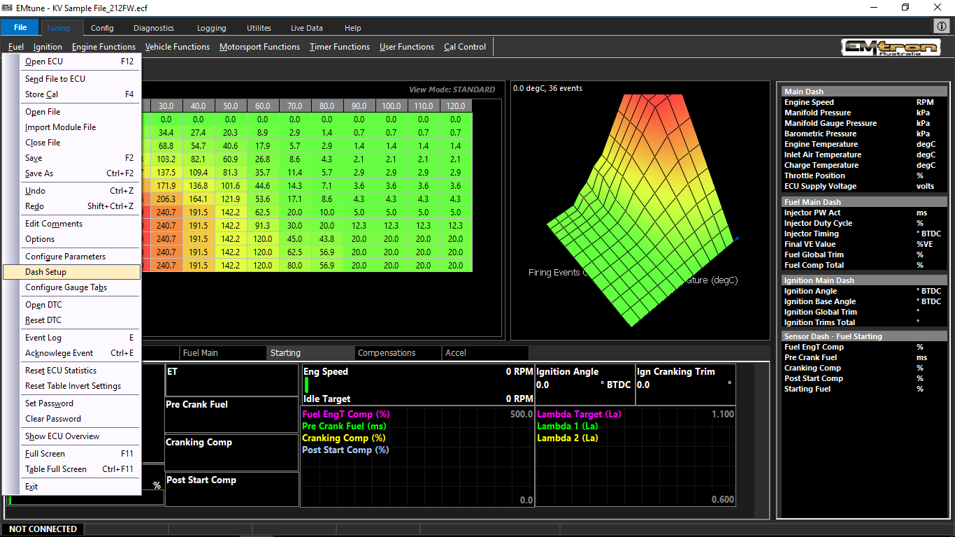
The entire dash layout can be imported and exported via that “Dash Setup” selection under the file menu.
** Periodically save your dash setup
Emtune Welcome Screen
Welcome Screen
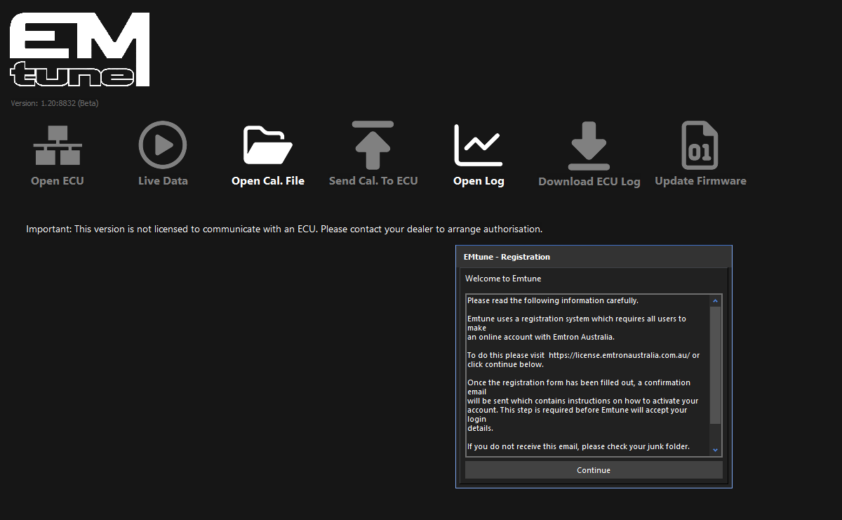
When first opening Emtune software a Welcome Screen is displayed.
From here the user has several options in which they would want to use the connection to their PC.
This is one of the unique features to Emtron/Emtune as it eliminates many of the anxieties of connecting to ECU systems.
An end user can easily download an ECU log, or look at one way Live Data communication without actually opening the calibration file.
Open ECU
Only available when ECU is connected
Use this option to connect to the ECU to perform configuration, calibration, live PC data logging, scope functions, and more.
This is the main mode for live calibrating.
Tuning Tip: The Hot key to achieve connection / disconnection lieu of using the mouse is F12
Live Data
Only available when ECU is connected
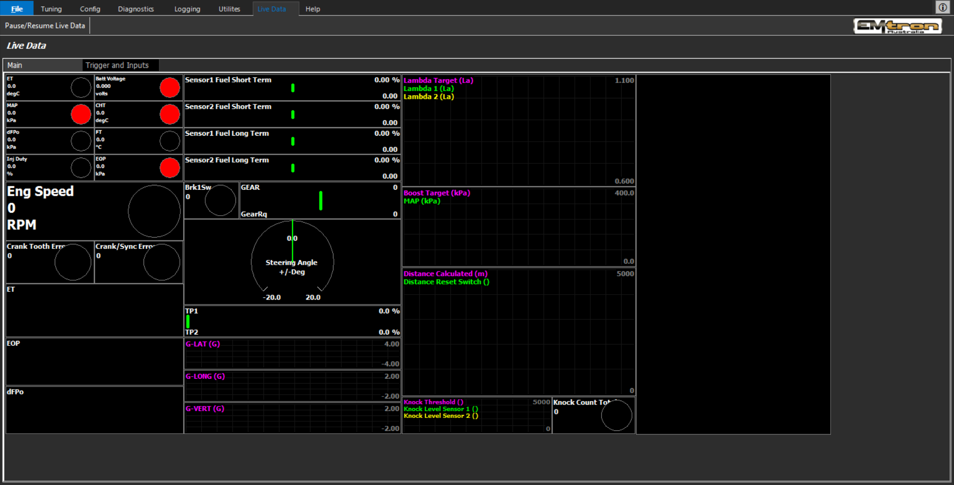
This option allows the user to connect to the ECU in a “one way” communication mode. The mode does not allow transmitting of any user settings that can change the calibration in any way. The live data display dashboards, runtime plots, gauges, pages, tabs, and more must be configured in the Open ECU/Open File modes. Generally this is performed by the dealer/installer/calibrator of the ECU as depending on the application the display changes may change. All runtime data is also available in the Live Data mode as well.
Open File
Available anytime the software is opened
This mode allows offline calibration editing, as well as configuration of the Live Data page.
Send File to ECU
Only available when ECU is connected
A previously saved calibration file (either from live calibrating, or offline editing) can be sent and stored to the ECU with this option. This allows the user to update the calibration file without having to open the ECU.
Update Firmware
Only available when ECU is connected
Use this function to update the ECU Firmware.
CautionThis procedure should only be done by authorized dealers unless under strict instruction to do so otherwise. The ECU should have a stable power source during updating as it takes up to 25 min to complete.
Download ECU Log
Only available when ECU is connected
This function downloads the ECU log. The ECU logging function is configured in the Open ECU/Open File mode inside the calibration file.
Licence Expired
Licence Expired
Math Expressions
A user definable mathematical equation that allows the user to generate channels for data analysis or to aid in rapidly validation tuning data. The expression is defined by a single line of text that can include most common mathematical operations and many advanced functions.
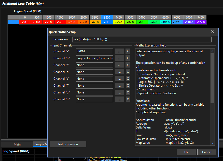
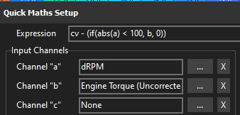
In the above example, the expression cv - (if(abs(a) < 100, b, 0)) is used.
When the Q key is pressed, the expression takes the current table cell value cv and subtracts Engine Torque (Uncorrected) b, but only if the absolute Derivative Engine Speed a is less than 100 RPM/s, otherwise it subtracts nothing. This means it will automatically fill in the frictional loss table for you but it makes sure the engine speed is stable.
Syntax
Spaces are ignored by the compiler and can be omitted or included to improve readability. There is no difference to the result.
Operator / Character
Description
Usage
Example
Result
Arithmetic
+
Add
x + y
12 + 3
15
-
Subtract
x - y
12 - 3
9
*****
Multiply
x * y
12 * 3
36
/
Divide
x / y
12 / 3
4
%
Modulus / Remainder
x % y
12 % 3 12 % 10
0 2
******
Power
x ** y
12 ** 3
1728
Logical
<
Less Than
x < y
12 < 3 12 < 34
0 (false) 1 (true)
>
Greater Than
x > y
12 > 3 12 > 34
1 (true) 0 (false)
==
Equal To
x == y
12 == 3 12 == 12
0 (false) 1 (true)
!=
Not Equal To
x != y
12 != 3 12 != 12
1 (true) 0 (false)
<=
Less Than or Equal To
x <= y
12 <= 3 12 <= 34
0 (false) 1 (true)
>=
Greater Than or Equal To
x >= y
12 >= 3 12 >= 34
1 (true) 0 (false)
&&
And
x && y
12 && 3 1 && 0 0 && 0
1 (true) Both sides are non zero 0 (false) 0 (false)
**
**
Or
x
!
Negation
x = !y
x = !1 x = !0
x = 0 x = 1
Bitwise
«
Shift Left
x « y
56 « 2
224
»
Shift Right
x » y
56 » 2
14
&
Bitwise And
x & y
56 & 15
8
**
**
Bitwise Or
x
y
^
Bitwise XOR Bitwise Not (32 bit signed integer)
x ^ y ^x
56 ^ 15 ^56
55 -57
Other
=
Assignment
x = y
x = 5
Assigns value of 5 to variable “x”
,
Comma. Separates expressions or function arguments
x = y, x * z min(x, y)
x = 5, x * 2 min(12, 3)
10 3
Variables
The letters a through h can be user assigned to any loggable ECU runtime parameter. These variables can then be used anywhere in the expression. The user assigned variables are updated with the current parameter value every time the expression is evaluated.
Some other variables such as “pi” are pre-assigned for use in the expression.
Variable
Type
Note
User Variables
a
Assignable Input Parameter
b
Assignable Input Parameter
b
Assignable Input Parameter
c
Assignable Input Parameter
d
Assignable Input Parameter
e
Assignable Input Parameter
f
Assignable Input Parameter
g
Assignable Input Parameter
h
Assignable Input Parameter
Time
t
Time (seconds)
Calculated Channels Only
dt
Delta Time (seconds)
Calculated Channels Only
Constants
pi
Constant
Special
cv
Cell Value
Table Math Only. Represents the value of the table cell before any math operation is performed.
It’s possible to create and assign variables within the expression. This can be useful for breaking up the expression to make it more readable.
For example these two expressions are functionally equivalent:
cv *max(a, b, c, d)
m =max(a, b, c, d), cv * m
Here two separate operations are created and separated by the comma character. First a variable called m is created and assigned the result of the max() function. Secondly the table cell cell value cv is multiplied by m. As there is no more work to do the expression returns the result of the second operation which then gets passed to the table to be used.
Variables can remember their value between iterations:
x = x +1
The variable x is created and incremented by 1 every time the expression is evaluated.
y =5, x = x + y
The variable y is created and assigned the constant value of 5. With every evaluation, x is increased by the value of y which in this case is 5.
NOTE: The iterative nature of variables should be considered when writing expressions that may use them.
Functions
Functions are purpose built computational blocks that take input arguments to output a result. Functions are called by their name followed by brackets containing a list of arguments separated by commas. For example:
result =func(arg1, arg2, arg3)
Some functions take a single input argument, some take more. Arguments can be any other valid syntax type such as constants, variables, other functions or logic expressions.
See the table below for a list of the available functions and their usage.
*Optional Argument
Function Abbreviation
Full Name
Description
Arguments
Example
abs(x)
Absolute
Returns the absolute (positive) value of the input. Turns a negative value into a positive. Makes no change to a value that is already positive.
1. x Input value
abs(123) = 123 abs(-123) = 123
acu(x, t)
Accumulator
Time based average of 100 evenly spaced samples taken over the given time ’t’ in seconds.
1. x Input value 2. t Time (seconds)
acu(a, 10) Returns the average of the last 10 seconds worth of the variable ‘a’. Can be used to generate accumulated load values from parameters such as Manifold Pressure or Throttle Area Demand.
av(x, y, z, *…)*
Average
Averages the values of all given inputs. Requires 2 or more inputs.
1. x Input Value 1 2. y Input Value 2 3. zOptional. Input Value 3 And so on…
av(a, b) Returns the average of inputs ‘a’ and ‘b’. av(a, b, c, d, e, f) Returns the average of inputs ‘a’, ‘b’, ‘c’, ’d’, ’e’, ‘f’. av(123, 45, 67) Returns 78.333
dv(x, ti)
Delta Value
Calculates the rate of change in the input value over per second. Samples are taken at the specified time interval. The output is expressed in units per second.
1. x Input Value 2. ti Time Interval (seconds)
dv(a, 0.2) Suppose ‘a’ was 10 at the previous sample. Now, 0.2 seconds later the value of a is 15. ‘a’ has changed by +5 over 0.2 seconds. The result will be 5 / 0.2 = 25 or 25 units per second.
if(cond, true, false)**
If
Performs Logical evaluation and either outputs a boolean (0 or 1) result or it outputs the optionally provided true/false values. The function checks the value of the first argument (cond). If the value is greater than 0 then it will either return the value passed in to the second argument (true) or 1. If the cond value is 0, then it will either return the value passed in to the third argument (false) or 0.
1. cond Input condition. Can be any variable, function or logic expression. 2. true Optional#8202;.* This value is returned by the if() function when the input condition evaluates to greater than 0. If a true argument is not provided, the true result defaults to 1. 3. false* Optional. This value is returned by the if() function when the input condition evaluates to zero. If a false argument is not provided, the false result defaults to 0.
if(a > b) Only argument 1 provided. If the value of channel ‘a’ is greater than the value of the channel ‘b’ then the function will output 1, else it will output 0. if (a, b) Arguments 1 & 2 provided. If the value of channel ‘a’ is greater than 0, then the result will be the value of channel ‘b’, else 0 (as no 3rd argument for false is given). if(a ** 2 == 9, 10, b + 1) Arguments 1, 2, & 3 provided. If the value of the channel ‘a’ squared is equal to 9, then the result is 10, else the result is the value of channel ‘b’ plus 1.
lim(x, min, max)
Limit
Clamps the input value to the given range limits.
1. x Input Value 2. min Minimum allowed output 3. max Maximum allowed output
lim(a, 10, 90) If ‘a’ is less than 10, the output will be 10. If ‘a’ is greater than 90, the output will be 90. If ‘a’ is within the range of 10 to 90, the output will be ‘a’ unchanged.
lp(x, α)
Low Pass Filter
A simple low pass filter. Output = (α % of the filtered value) + (100 - α % of the new value)
1. x Input Value 2.α Alpha (%)
lp(a, 85) Suppose ‘a’ has a current filtered result of 95. Now the filter is given the new value of 100. The new filtered result = (95 * 0.85) + (100 * 0.15) = 80.75 + 15 = 95.75. The filter will now store 95.75 as the previous result and return 95.75 as the output. If the input was to stay at 100, after several iterations the output will arrive at 100 also.
map(x, x1, x2, y1, y2)
Map / Interpolate
Linearly Maps/Interpolates the input value to a new range of output values. For example if x values are voltage and y values are percentages, the function would interpolate the input voltage to the spanned output percentage.
1. x Input Value 2. x1 Input Range Position 1 3. x2 Input Range Position 2 4. y1 Output Range Position 1 5. y2 Output Range Position 2
map(a, 0.5. 4.5, 0, 100) If ‘a’ is 0.5, the output will be 0. If ‘a’ is 4.5 the output will be 100. If ‘a’ is 2.0, the output will be 37.5. If ‘a’ is 0.2 the output will be -7.5. If ‘a’ is 4.8 the output will be 107.5.
mapl(x, x1, x2, y1, y2)
Map / Interpolate (Limited)
Similar to map() however the output result is clamped to the y1, y2 range limits.
1. x Input Value 2. x1 Input Range Position 1 3. x2 Input Range Position 2 4. y1 Output Range/Limit Position 1 5. y2 Output Range/Limit Position 2
mapl(a, 0.5. 4.5, 0, 100) If ‘a’ is 0.5, the output will be 0. If ‘a’ is 4.5 the output will be 100. If ‘a’ is 2.0, the output will be 37.5. If ‘a’ is 0.2 the output will be 0. If ‘a’ is 4.8 the output will be 100.
max(x, y, z, …*)*
Max Value
Returns the highest of any of the given input values. Requires 2 or more inputs.
1. x Input Value 1 2. y Input Value 2 3. zOptional. Input Value 3 And so on…
max(a, b) Returns the maximum of inputs ‘a’ or ‘b’. max(a, b, c, d, e, f) Returns the maximum of inputs ‘a’, ‘b’, ‘c’, ’d’, ’e’, ‘f’. max(123, 45, 67) Returns 123
min(x, y, z, …*)*
Min Value
Returns the lowest of any of the given input values. Requires 2 or more inputs.
1. x Input Value 1 2. y Input Value 2 3. zOptional. Input Value 3 And so on…
min(a, b) Returns the maximum of inputs ‘a’ or ‘b’. min(a, b, c, d, e, f) Returns the maximum of inputs ‘a’, ‘b’, ‘c’, ’d’, ’e’, ‘f’. min(123, 45, 67) Returns 45
sqrt(x)
Square Root
Calculates the square root of the input value.
1. x Input Value
sqrt(a) Returns square root of a sqrt(123) Returns 11.0905365
sin(x)
Sine
Calculates the Sine of the input value.
1. x Input Value
sin(a) Returns sine of a sin(123) Returns 0.83867
cos(x)
Cosine
Calculates the Cosine of the input value.
1. x Input Value
cos(a) Returns cosine of a cos(123) Returns -0.544639
tan(x)
Tangent
Calculates the Tangent of the input value.
1. x Input Value
tan(a) Returns tangent of a tan(123) Returns -1.539865
Examples
VE Table Quick Validate
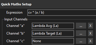
cv * (a / b)
a = Lambda Avg
b = Lambda Target
This is equivalent to the operation performed when pressing the L key during live tuning. The advantage here is that the the expression can be performed using the the current log cursor position values as inputs.
Bank 1 Trim Table Quick Validate
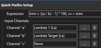
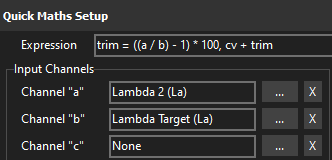
trim = ((a / b) -1) *100, cv + trim
a = Lambda 1*
b = Lambda Target*
Similar to the VE expression except that it gives a percentage offset value to be used in the bank trim table. Assumes Bank 1 is measured by Lambda 1.
First the trim is calculated, then the trim is added to the cell value
Bank 2 Trim Table Quick Validate
trim = ((a / b) -1) *100, cv + trim
a = Lambda 2
b = Lambda Target
Similar to the VE expression except that it gives a percentage offset value to be used in the bank trim table. Assumes Bank 2 is measured by Lambda 2
Frictional Loss Table
cv - (if(abs(a) <100, b, 0))
a = dRPM
b = Engine Torque (Uncorrected)
When the engine is accelerating, torque is positive. When the engine is decelerating torque is negative. When the the engine speed is stable (unloaded free revving) the torque is 0. The frictional loss table is used to account for the internal drag of the engine rotating assembly in order to give the correct 0mn final torque value.
The expression checks the dRPM to make sure the engine is held at a near constant RPM (less than a generous 100 rpm/s in this example) where final torque should be 0nm. The abs() function is used to turn a negate dRPM value into a positive to simplify the < (less than) logic. If the dRPM check is true, the current Engine torque value is subtracted from the cell value, if not 0 is subtracted from the cell value, ie. nothing happens.
Calculated Channels
Extreme Example: Knock Threshold Level Helper
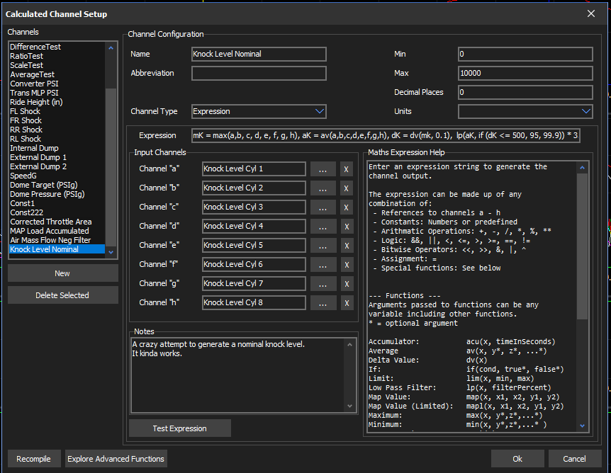
mK =max(a,b,c,d,e,f,g,h), aK =av(a,b,c,d,e,f,g,h), dK =dv(mk, 0.1), lp(aK, if (dK <=500, 95, 99.9)) *3.2
a - h = Knk Level Cyl #
An example of using some nested expressions to generate a bit of an idea of what the ideal knock threshold value might be.
The expression finds the max knock (mK), then the average knock (aK), then the derivative of the max over 100ms. Next applies a low pass filter over the average, and adjusts the filter level depending on the derivative. Finally it multiplies the result by 3.2.
This is an example only and isn’t intended to be useful as is for any or all applications. It does however show how functions and variables can be nested in a variety of ways.
Store Cal (F4)
The Store Cal function stores the Cal File to the ECU permanently.
It is also accessible by the F4 hotkey or from the File Tab.
Warning: Failure to Store Cal after making changes will result in lost of data.
Tips & Tricks
Tips on Improving your Emtune tuning efficiency…
Methods of validating VE Table
Auto Lambda Correction:
Utilise “L” Auto Lambda Correction feature of the software.
“L” applies current Lambda Target Error % to live location in map automatically.
Manual Entry Lambda Correction:
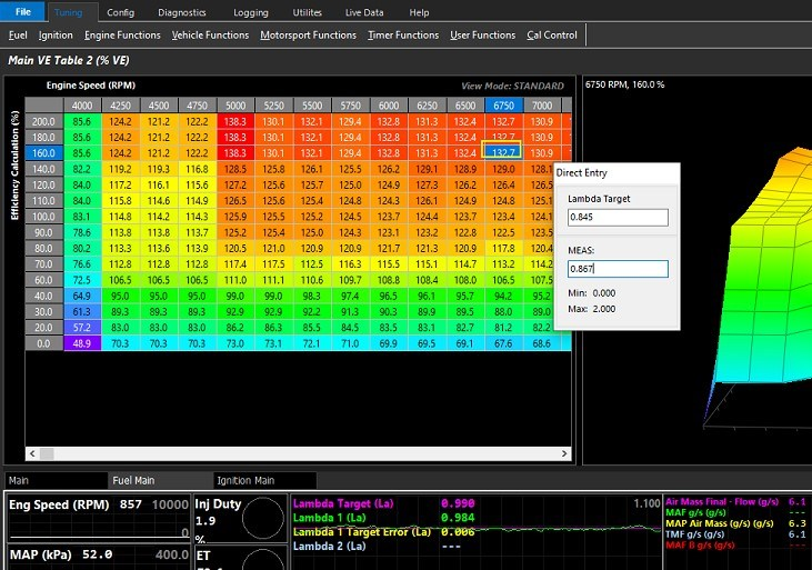
Using “M” key “Manual Entry Lambda correction method”.
“M” is pressed & the Lambda target value is imputed together with the measured value. Enter and the result is applied to the highlighted cell.
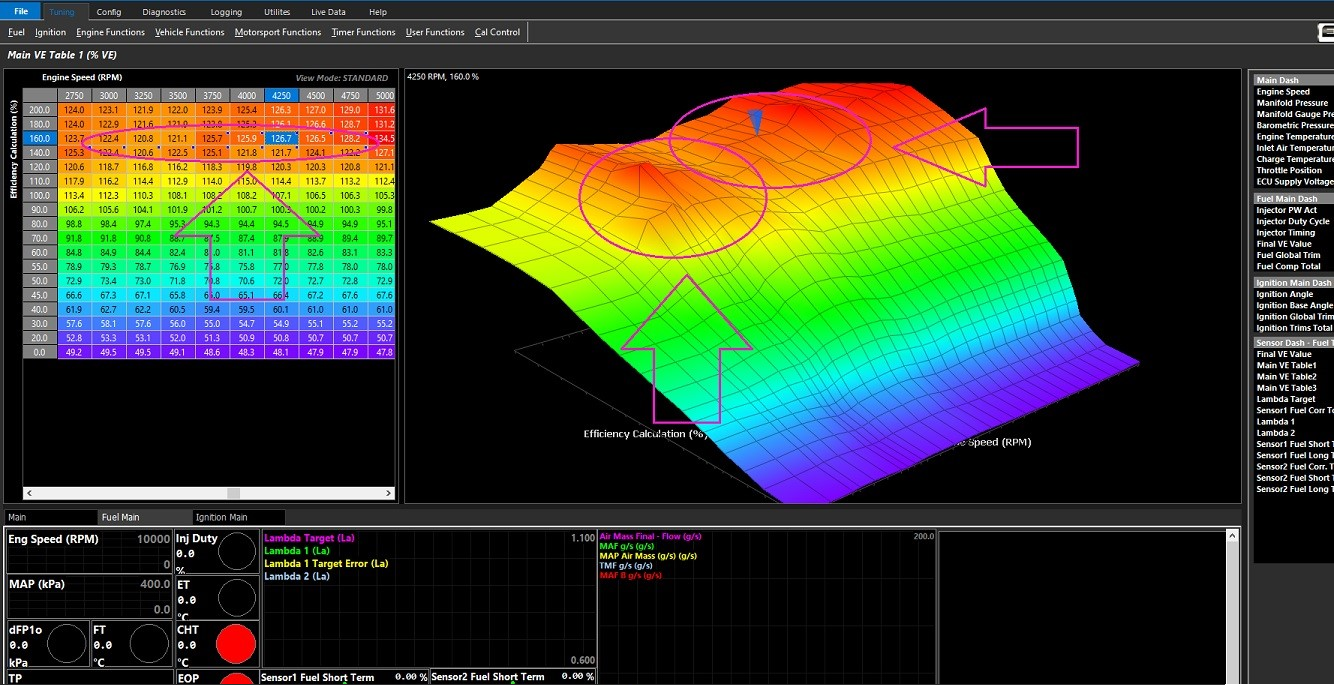
Direct Entry Lambda Correction
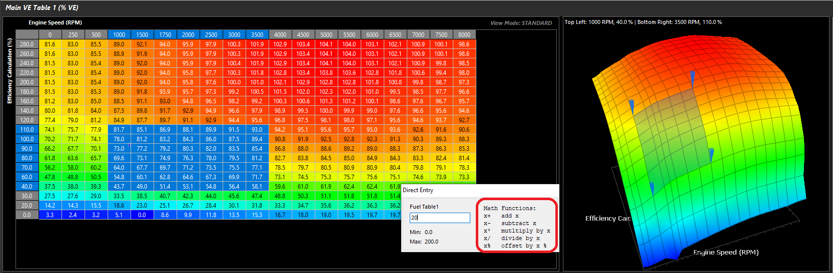
The maths value supplied in the target error runtime can be applied to the VE table as you would when using an excel spreadsheet, thereby correcting it. The table is highlighted & the correction manually entered.
Direct entry VE Correction Manual Maths examples:
Rich condition:
Lambda target: 0.864
Lambda 1: 0.782
Lambda Target error: 0.082
Highlight the cell to be corrected – Type 1.082 “/ “
Positive target error = division factor
Lean Condition:
Lambda target: 0.845
Lambda 1: 0.902
Lambda Target error: -0.057
Highlight the cell to be corrected – Type 1.057 “*” (Shift 8)
Negative target error = multiplication factor
Your goal should be to efficiently eliminate or minimise the error between the VE table & the Lambda target table.
Tip: To use this feature & validate the VE table, alter the dashboard to show not only the Lambda Target and Lambda 1/2, but also the Lambda Target Error.
Utilising “P” key (Pause)
Tuning tables can be quickly validated by utilising the “P” key to pause the live logging in the dashboard independent of the PC logging. This will allow you to drive through an area of a particular table, press “P” & then come back & edit where you have been.
Double clicking the mouse over the desired dashboard runtimes will allow you to move left & right through the paused data using the left & right arrow keys & will also highlight (overlay) the cells referenced in the table being validated.
“L”, “M”, and Table Maths are all available and usable as if being utilized “live” wherever the cursor is “paused”
Live logging recommences when “P” is pressed for the 2nd time.
Utilising “O” Toggle Logger Position (The Yellow Box)
Using the PC logger (F8) the tune can be interrogated against target tune parameters.
Note: Setup your logger view to show the Lambda Target Error not found in default logger layout.
Once an area has been identified that needs attention.
The cursor is moved to highlight this area.
Returning to the referenced VE table in the tuning software.
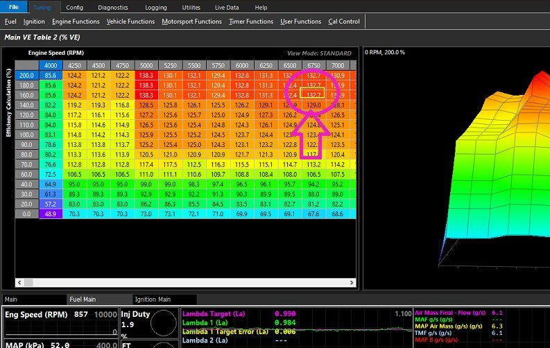
Pressing “O” will toggle the yellow box over the referenced cell/s.
Lambda vs Lambda target can be utilised via “M” - Manual entry lambda correction.
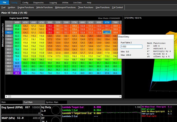
Or direct entry method can be utilised.
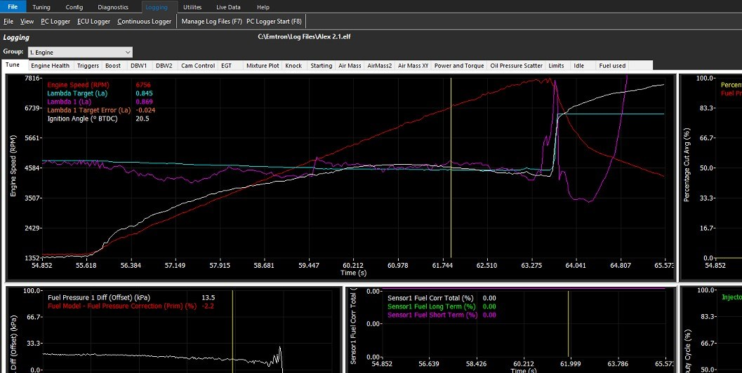
Working example:
Lambda Target is 0.845
Lambda 1 (La) is 0.867
Lambda 1 Target Error (La) is -0.022 % (Lean)
To correct the table simple left mouse, click the referenced cell
Start typing 1.022* (shift 8)
This multiplies the missing percentage of fuel into the VE table thereby validating the table.
Maths values are explained in dropout box once typing commences.
(Rich values are divided)
Your goal should be to efficiently eliminate or minimise the error between the VE table & the Lambda target table.
Utilising “Scatter Plot” Correction
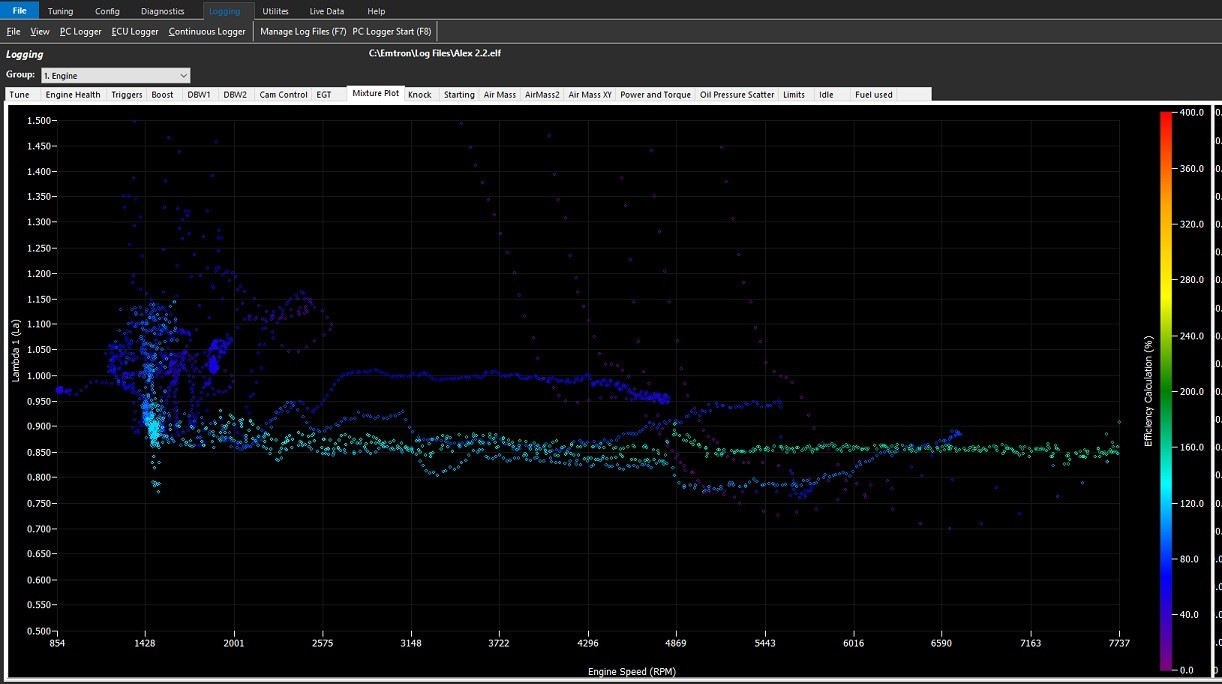
A useful feature of the Emtune logging is the Mixture Scatter Plot.
This is an often overlooked powerful and accurate tool for validating your VE table/s.
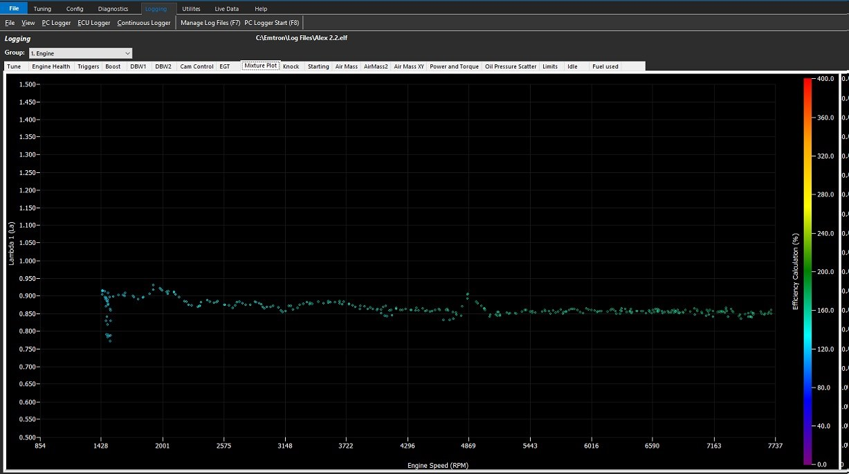
By utilising the features of the setup, this table can be utilised as a form of histogram of engine operation.
Note: Scatter plot correction applications are not limited to only VE tables. This method of validation is easily applied to bank trims & more.
Example: Lambda 1 active / Lambda control off
Validation performed on chassis dyno
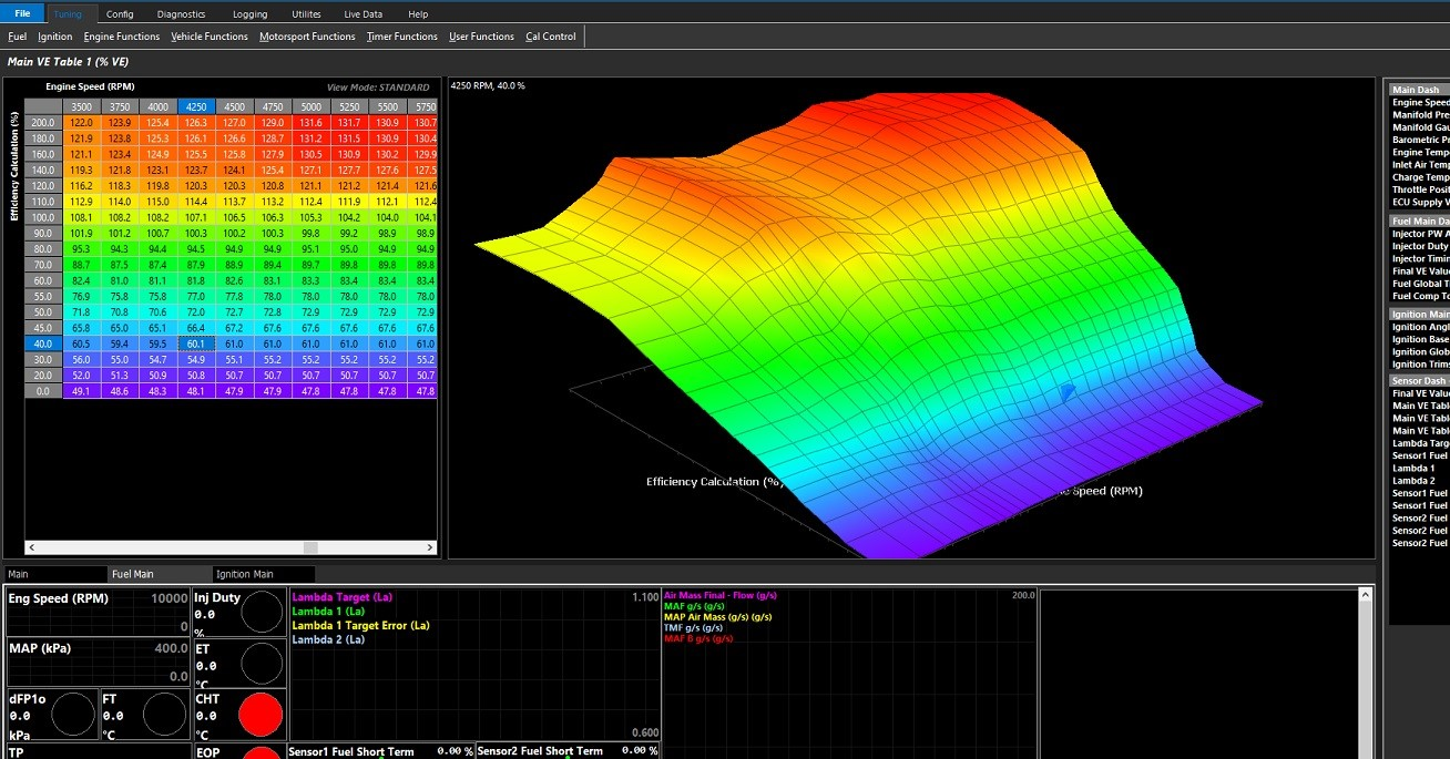
VE Table for purpose of demonstration
The vehicle is driven and a PC log is produced recording the activity
Raw scatter plot is produced
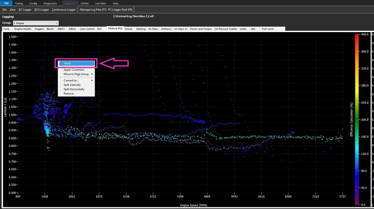
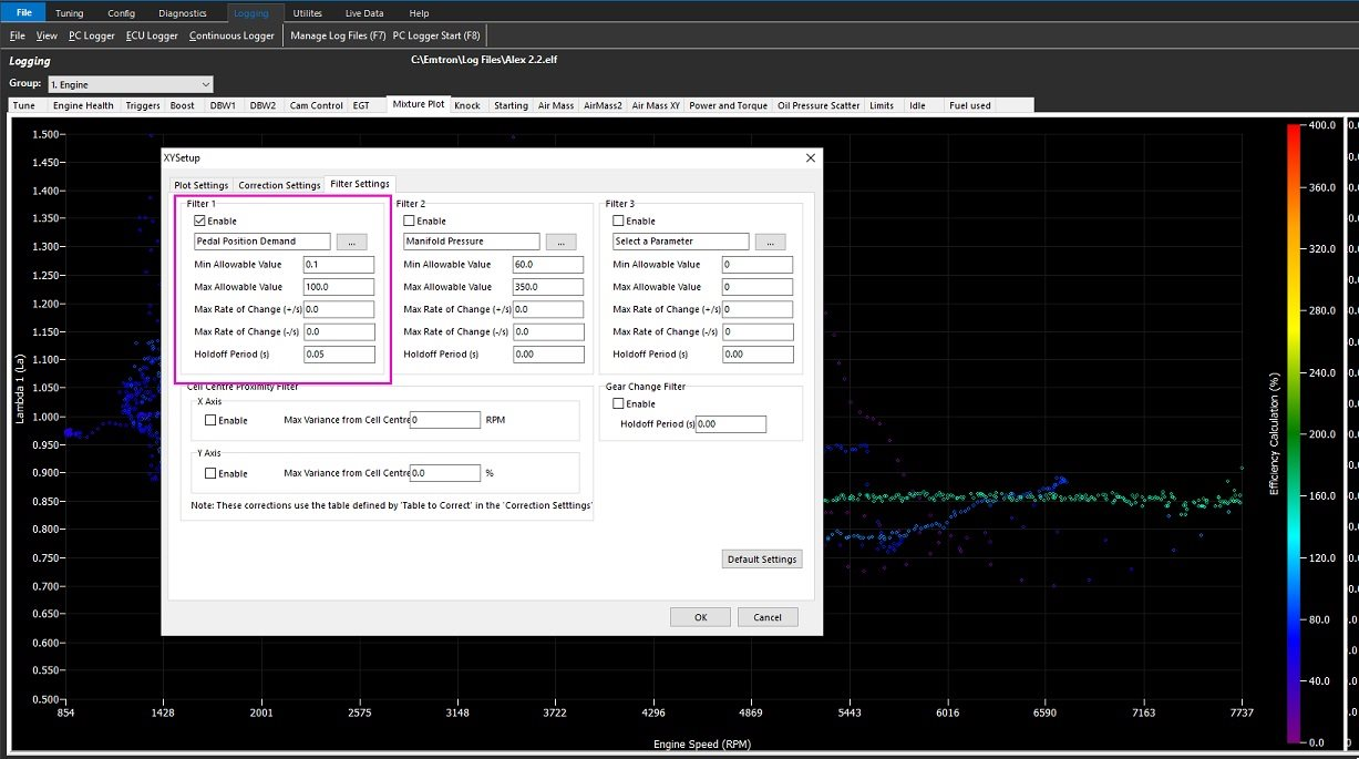
Enter the Scatter Plot Setup (Right Mouse Click)
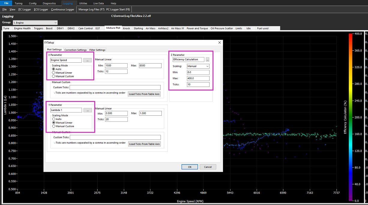
Confirm Plot Settings
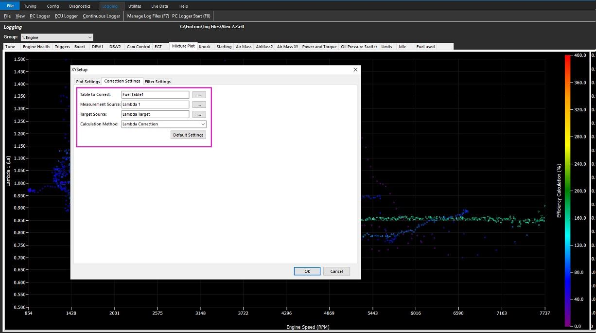
Confirm Correction Settings
Set appropriate filters as required
Return to the filtered scatter plot
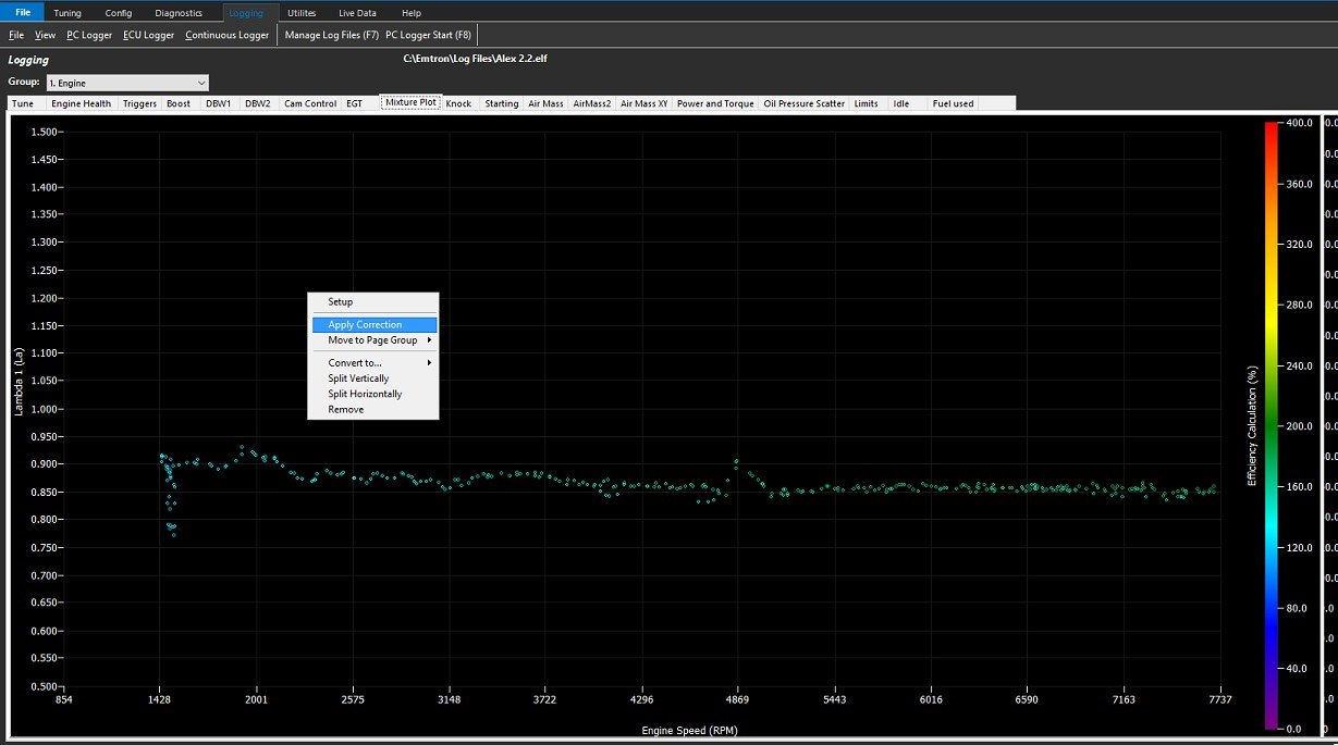
Apply the correction
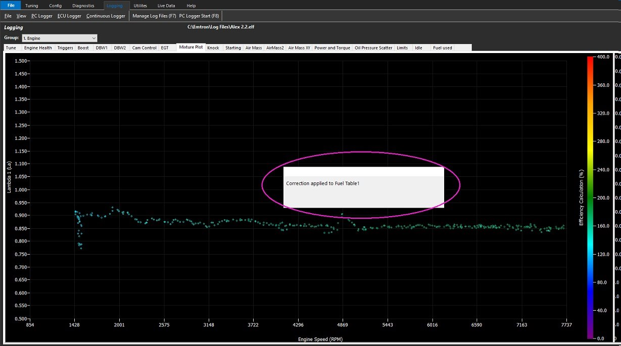
Emtune with acknowledge when this is complete
Tuning
Software Navigation
From the Welcome Screen, selecting Open File, or Open ECU (ECU Detected is required) the calibration file will be opened.
From here, you can navigate through a number of menus, tabs, sub tabs, etc.
The Emtune software has a very systematical approach to configuration.
Start on the left side, and work your way over from left to right.
Do not skip sections. Following this practice as accurately as possible will ensure tuning process will move smoothly in the future.
** Tuning should only be done once Basic Configuration and ECU Setup is complete (Config) - See Basic Configuration
*** If Tuning Functions are not available, it is due to the Configuration not being completed (see Config)
Table tools/maths
Several hotkeys and shortcuts are available in all tables to make management of entering values quick and easy.
Hotkeys PgUp/PgDwn will increase and decrease cells. Holding shift key will increase/decrease values faster.
Using the mouse, you can select multiple cells, to change multiple cells at a time, or use the keyboard while holding the CTRL key.
With cells selected, you can:
Increase/Decrease incrementally using PgUp/Down (holding shift key will increase/decrease values faster)
Interpolate between cells using keys I, R, C (I will interpolate diagonally, R horizontally - row, C vertically - column)
Or use table maths. Typing numbers into the keyboard will allow you to add, subtract, multuply, divide, or increase/reduce %.
Selecting a lot of cells, also holding the CTRL key, allows you to drag them around with the arrow keys to move them around the table (so easily move a line/section around the map).
Right clicking the table shows options for hot keys mentioned above, but also the ability to Save Table externally, Load table from a separate file, but also import table.
Importing a table allows you to select another calibration file, and the software will reference the cal file selected, and grab the table from that location for the current working cal file.
This is a useful tool when building new calibrations if the user is trying to bring over certain tables that mostly will cross over.
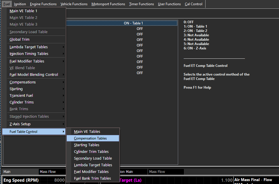
**** If Compensation (or other) Tables are not available, they must be enabled within the specific sub menu -> Fuel -> Fuel Table Control
Fuel
Fuel section allows the user to tune multiple tables for air flow , user compensations, air and fuel mass modifiers, Lambda Target, and more.
Some noteworthy functions are :
Charge Temperature Estimation
To properly estimate actual “inlet air temperature”, the Emtron will generate a channel called “Charge Temperature”, which is calculated and offset based on a number of variables.
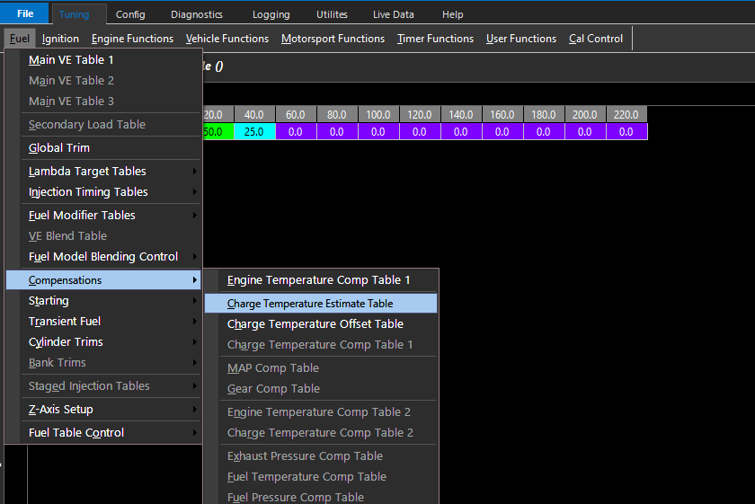
The Charge Temperature Estimation table is available under Tuning -> Fuel -> Compensations -> Charge Temperature Estimation
A value of 100 will set the Charge Temperature as Engine Temperature (commonly water temp), and a value of 0 will set the Charge Temperature as Inlet Air Temperature.
A careful blending of these values will allow the user to properly estimate the charge temperature going into the engine under varying loads to anticipate heat soak scenarios, and eliminate error from the engine model.
** See KV Sample file for an example of of how the Charge Temperature Estimate Table can be used.
Charge Temperature Offset
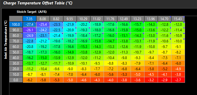
The Charge Temperature Runtime can also be “offset” by a table under Tuning -> Fuel -> Compensations -> Charge Temperature Offset
The purpose of this table allow the Charge Temperature runtime to gain greater accuracy based on any other variables the user deems necessary
The most common use of this table is to account for charge cooling based on fuel injected in the engine as shown above, where the ECU is using “Stoich Target”, that is a runtime generated by the ECU using the current Stoich value multiplied by the live Lambda Target value (therefore current Air to Fuel Ratio). The fuel type being used for example can vastly affect the actual AFR and subsequently offset the actual Charge Temperature
The Air to Fuel Ratio in this instance is relative to charge cooling, and how this table is being built.
Ignition
Ignition section allows the user to tune multiple tables regarding ignition control
Some noteworthy functions are :
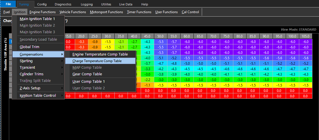
Charge Temperature Comp Table
As mentioned in the fuel section, due to some differences in how the Charge Temperature channel is calculated in the Emtron model (particularly how it is offset-ted in the Charge Temperature Offset Table), this table must have special attention as the values for Charge Temperature may not be what the user is “used” to.
** The values may be much lower where ignition compensation must be applied than normal vs compensating using standard Inlet Air Temperature
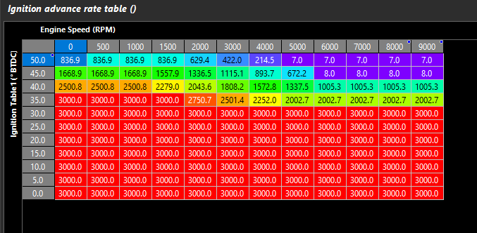
Ignition Advance/Retard Rate Tables
These tables located under Tuning -> Ignition -> Transient are always active
They dictate how quickly the ignition advance can be changed, and a table can be generated to slow/speed up the advance/retard rate.
The values are in degrees/second. Maximum values are 3000 degrees/second.
Engine Functions
Engine Functions section allows the user to tune functions related to “Engine”, such as throttle body, torque, idle speed, drive by wire, etc.
Some noteworthy functions are :
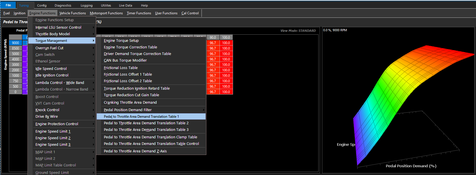
Torque Management
The Torque Management section allows the user to dictate various torque settings.
One main difference is if Drive By Wire throttle is used, the targeting structure is based on a Pedal Demand -> Throttle area function.
Please see the Drive By Wire, Throttle Body Model, and Torque Management sections for more help on these sections.
Vehicle Functions
Vehicle Functions section allows the user to tune functions related to “Vehicle”, such as EFI Relay Control, Cooling Fan, Fuel Pumps, Air Con, etc.
Some noteworthy functions are :
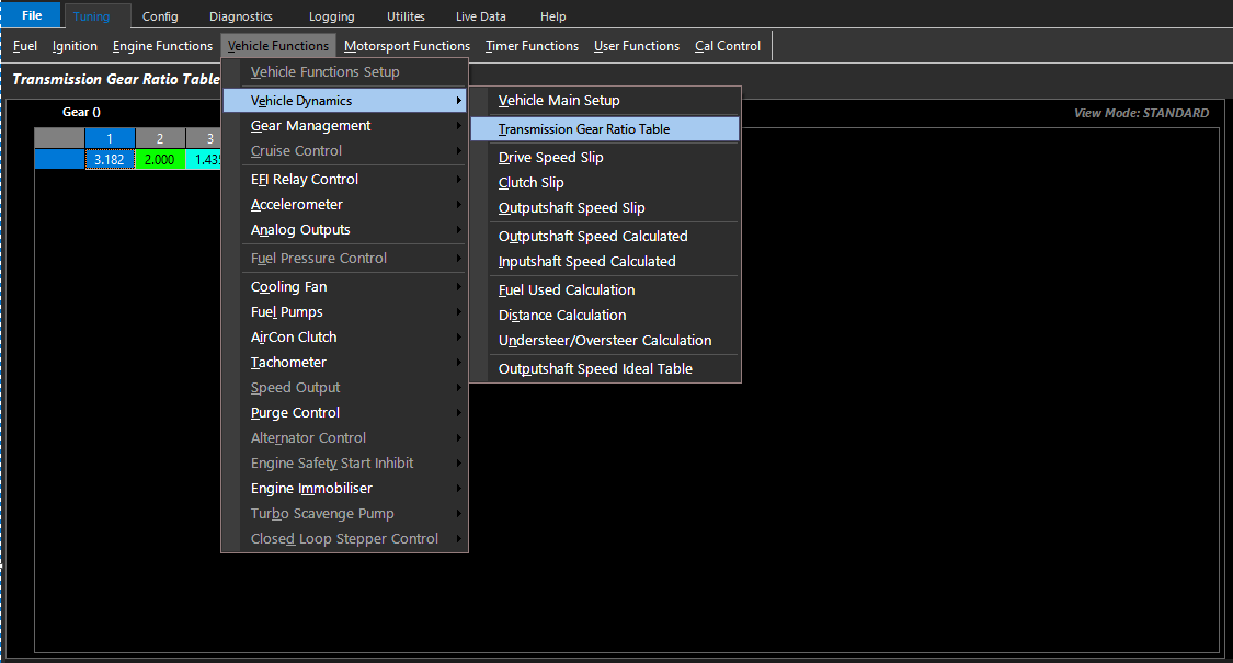
Vehicle Dynamics
Vehicle Dynamics section allows the user to dictate wheel sizes, gear ratios, slip channels, etc.
For advanced Motorsport Functions to correctly operate, these settings must all be properly configured.
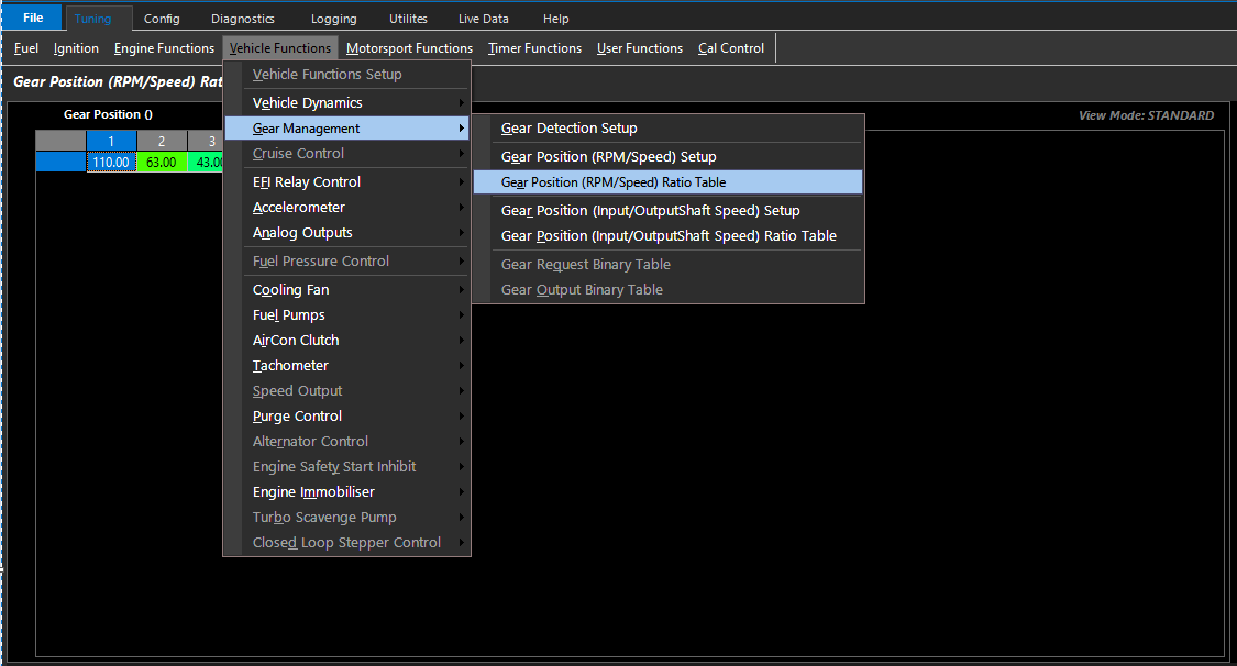
Gear Management
Emtron has multiple methods of Gear Detection. In this section, these detection methods can be configured.
** In order for Motorsport Functions to correctly operate, these settings must all be properly configured.
Motorsport Functions
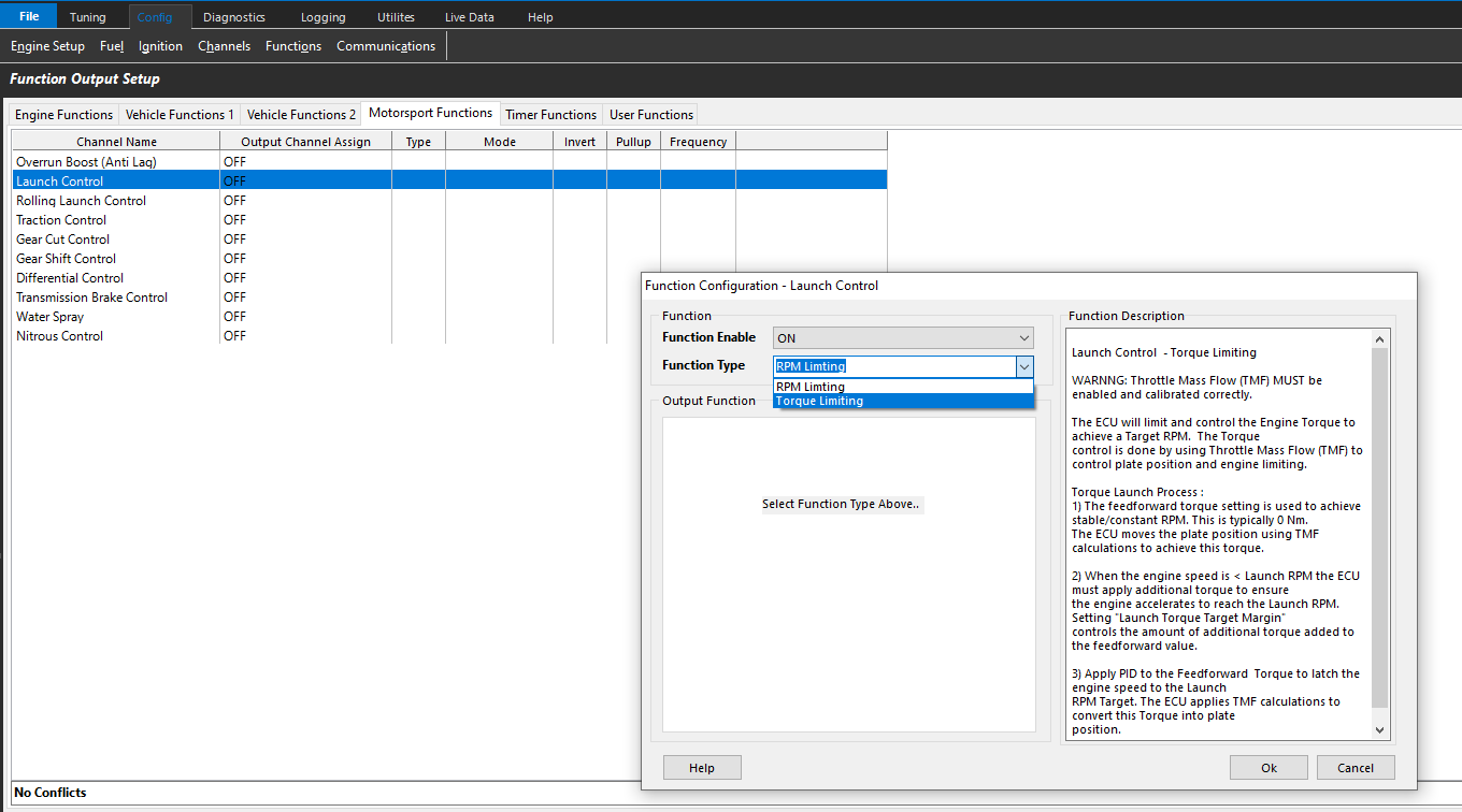
Motorsport Functions section allows the user to tune functions related to “Motorsport”, such as Anti-Lag, Launch Control, Gearshift Control, Traction Control, etc.
Some noteworthy functions are and more complex functions are listed below simply as a preview of these complex functions :
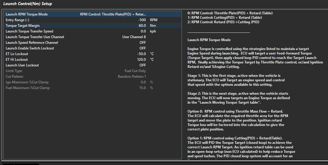
When selecting Torque Limiting Launch Control, multiple types of Torque Limiting Launch are available under the tuning tab
See Launch Control Help section for more details on different Launch Control Programs
Gearshift Control
Emtron can control multiple types of Gearshift Control (mechanical gear stick, paddle shift, etc). Once enabled, there are many settings to further refine gearshift functions and very specific and special runtimes available. This is one of the most flexible systems in the ECU.
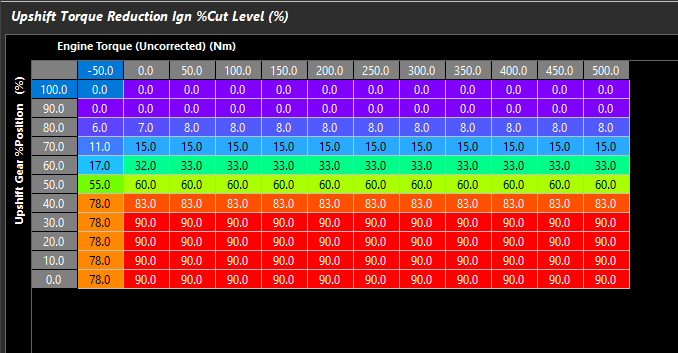
An example of “Upshift Gear %Position” which is the percentage between valid gear (between tolerance voltages if defined in the gear voltage input) being used to limit Ignition cut through a gearshift
Timer Functions
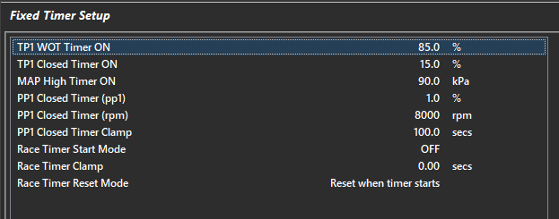
Timer Functions section allows the user to tune functions related to “Timers”. There are 5 user configurable timers, plus multiple standard timers, and a race timer.
These timers generate channels that can be used in the ECU in tables, functions, etc.
User Functions
There are 10 User Functions that allow the user to create universal functions in the ECU.
These functions have multiple conditions to make them active, can be set up to run physical outputs (outputs assigned), or virtual outputs (outputs assigned as “On - No Output”), set as PWM, and even set as variable Frequency.
See Config -> Functions -> User Functions for more details on the flexibility of these functions
** User Function Output status and Duty Cycle runtimes are available to be used furthermore in other locations in the ECU.