Math Expressions
A user definable mathematical equation that allows the user to generate channels for data analysis or to aid in rapidly validation tuning data. The expression is defined by a single line of text that can include most common mathematical operations and many advanced functions.
 In the above example, the expression
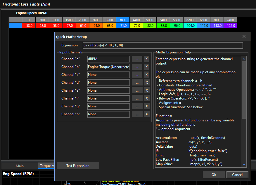
 cv - (if(abs(a) \< 100, b, 0)) is used.
When the Q key is pressed, the expression takes the current table cell value cv and subtracts Engine Torque (Uncorrected) b, but only if the absolute Derivative Engine Speed a is less than 100 RPM/s, otherwise it subtracts nothing. This means it will automatically fill in the frictional loss table for you but it makes sure the engine speed is stable.
Syntax
Spaces are ignored by the compiler and can be omitted or included to improve readability. There is no difference to the result.
| Operator / Character | Description | Usage | Example | Result |
|---|---|---|---|---|
| Arithmetic | ||||
| + | Add | x + y | 12 + 3 | 15 |
| - | Subtract | x - y | 12 - 3 | 9 |
| * | Multiply | x * y | 12 * 3 | 36 |
| / | Divide | x / y | 12 / 3 | 4 |
| % | Modulus / Remainder | x % y | 12 % 3 12 % 10 | 0 2 |
| ** | Power | x ** y | 12 ** 3 | 1728 |
| Logical | ||||
| < | Less Than | x < y | 12 < 3 12 < 34 | 0 (false) 1 (true) |
| > | Greater Than | x > y | 12 > 3 12 > 34 | 1 (true) 0 (false) |
| == | Equal To | x == y | 12 == 3 12 == 12 | 0 (false) 1 (true) |
| != | Not Equal To | x != y | 12 != 3 12 != 12 | 1 (true) 0 (false) |
| <= | Less Than or Equal To | x <= y | 12 <= 3 12 <= 34 | 0 (false) 1 (true) |
| >= | Greater Than or Equal To | x >= y | 12 >= 3 12 >= 34 | 1 (true) 0 (false) |
| && | And | x && y | 12 && 3 1 && 0 0 && 0 | 1 (true) Both sides are non zero 0 (false) 0 (false) |
| || | Or | x || y | 12 || 3 1 || 0 0 || 0 | 1 (true) 1 (true) Either side is non zero 0 (false) |
| ! | Negation | x = !y | x = !1 x = !0 | x = 0 x = 1 |
| Bitwise | ||||
| << | Shift Left | x << y | 56 << 2 | 224 |
| >> | Shift Right | x >> y | 56 >> 2 | 14 |
| & | Bitwise And | x & y | 56 & 15 | 8 |
| | | Bitwise Or | x | y | 56 | 15 | 63 |
| ^ | Bitwise XOR Bitwise Not (32 bit signed integer) | x ^ y ^x | 56 ^ 15 ^56 | 55 -57 |
| Other | ||||
| = | Assignment | x = y | x = 5 | Assigns value of 5 to variable “x” |
| , | Comma. Separates expressions or function arguments | x = y, x * z min(x, y) | x = 5, x * 2 min(12, 3) | 10 3 |
Variables
The letters a through h can be user assigned to any loggable ECU runtime parameter. These variables can then be used anywhere in the expression. The user assigned variables are updated with the current parameter value every time the expression is evaluated.
Some other variables such as “pi” are pre-assigned for use in the expression.
| Variable | Type | Note |
|---|---|---|
| User Variables | ||
a | Assignable Input Parameter | |
b | Assignable Input Parameter | |
b | Assignable Input Parameter | |
c | Assignable Input Parameter | |
d | Assignable Input Parameter | |
e | Assignable Input Parameter | |
f | Assignable Input Parameter | |
g | Assignable Input Parameter | |
h | Assignable Input Parameter | |
| Time | ||
t | Time (seconds) | Calculated Channels Only |
dt | Delta Time (seconds) | Calculated Channels Only |
| Constants | ||
pi | Constant | |
| Special | ||
cv | Cell Value | Table Math Only. Represents the value of the table cell before any math operation is performed. |
It’s possible to create and assign variables within the expression. This can be useful for breaking up the expression to make it more readable.
For example these two expressions are functionally equivalent:
Here two separate operations are created and separated by the comma character. First a variable called m is created and assigned the result of the max() function. Secondly the table cell cell value cv is multiplied by m. As there is no more work to do the expression returns the result of the second operation which then gets passed to the table to be used.
Variables can remember their value between iterations:
The variable x is created and incremented by 1 every time the expression is evaluated.
The variable y is created and assigned the constant value of 5. With every evaluation, x is increased by the value of y which in this case is 5.
NOTE: The iterative nature of variables should be considered when writing expressions that may use them.
Functions
Functions are purpose built computational blocks that take input arguments to output a result. Functions are called by their name followed by brackets containing a list of arguments separated by commas. For example:
Some functions take a single input argument, some take more. Arguments can be any other valid syntax type such as constants, variables, other functions or logic expressions.
See the table below for a list of the available functions and their usage.
*Optional Argument
| Function Abbreviation | Full Name | Description | Arguments | Example |
|---|---|---|---|---|
| abs(x) | Absolute | Returns the absolute (positive) value of the input. Turns a negative value into a positive. Makes no change to a value that is already positive. | 1. x Input value | abs(123) = 123 abs(-123) = 123 |
| acu(x, t) | Accumulator | Time based average of 100 evenly spaced samples taken over the given time ’t’ in seconds. | 1. x Input value 2. t Time (seconds) | acu(a, 10) Returns the average of the last 10 seconds worth of the variable ‘a’. Can be used to generate accumulated load values from parameters such as Manifold Pressure or Throttle Area Demand. |
| av(x, y, z*, …*) | Average | Averages the values of all given inputs. Requires 2 or more inputs. | 1. x Input Value 1 2. y Input Value 2 3. z Optional. Input Value 3 And so on… | av(a, b) Returns the average of inputs ‘a’ and ‘b’. av(a, b, c, d, e, f) Returns the average of inputs ‘a’, ‘b’, ‘c’, ’d’, ’e’, ‘f’. av(123, 45, 67) Returns 78.333 |
| dv(x, ti) | Delta Value | Calculates the rate of change in the input value over per second. Samples are taken at the specified time interval. The output is expressed in units per second. | 1. x Input Value 2. ti Time Interval (seconds) | dv(a, 0.2) Suppose ‘a’ was 10 at the previous sample. Now, 0.2 seconds later the value of a is 15. ‘a’ has changed by +5 over 0.2 seconds. The result will be 5 / 0.2 = 25 or 25 units per second. |
| if(cond, true*, false*) | If | Performs Logical evaluation and either outputs a boolean (0 or 1) result or it outputs the optionally provided true/false values. The function checks the value of the first argument (cond). If the value is greater than 0 then it will either return the value passed in to the second argument (true) or 1. If the cond value is 0, then it will either return the value passed in to the third argument (false) or 0. | 1. cond Input condition. Can be any variable, function or logic expression. 2. true* Optional#8202;. This value is returned by the if() function when the input condition evaluates to greater than 0. If a true argument is not provided, the true result defaults to 1. 3. false* Optional. This value is returned by the if() function when the input condition evaluates to zero. If a false argument is not provided, the false result defaults to 0. | if(a > b) Only argument 1 provided. If the value of channel ‘a’ is greater than the value of the channel ‘b’ then the function will output 1, else it will output 0. if (a, b) Arguments 1 & 2 provided. If the value of channel ‘a’ is greater than 0, then the result will be the value of channel ‘b’, else 0 (as no 3rd argument for false is given). if(a ** 2 == 9, 10, b + 1) Arguments 1, 2, & 3 provided. If the value of the channel ‘a’ squared is equal to 9, then the result is 10, else the result is the value of channel ‘b’ plus 1. |
| lim(x, min, max) | Limit | Clamps the input value to the given range limits. | 1. x Input Value 2. min Minimum allowed output 3. max Maximum allowed output | lim(a, 10, 90) If ‘a’ is less than 10, the output will be 10. If ‘a’ is greater than 90, the output will be 90. If ‘a’ is within the range of 10 to 90, the output will be ‘a’ unchanged. |
| lp(x, α) | Low Pass Filter | A simple low pass filter. Output = (α % of the filtered value) + (100 - α % of the new value) | 1. x Input Value 2. α Alpha (%) | lp(a, 85) Suppose ‘a’ has a current filtered result of 95. Now the filter is given the new value of 100. The new filtered result = (95 * 0.85) + (100 * 0.15) = 80.75 + 15 = 95.75. The filter will now store 95.75 as the previous result and return 95.75 as the output. If the input was to stay at 100, after several iterations the output will arrive at 100 also. |
| map(x, x1, x2, y1, y2) | Map / Interpolate | Linearly Maps/Interpolates the input value to a new range of output values. For example if x values are voltage and y values are percentages, the function would interpolate the input voltage to the spanned output percentage. | 1. x Input Value 2. x1 Input Range Position 1 3. x2 Input Range Position 2 4. y1 Output Range Position 1 5. y2 Output Range Position 2 | map(a, 0.5. 4.5, 0, 100) If ‘a’ is 0.5, the output will be 0. If ‘a’ is 4.5 the output will be 100. If ‘a’ is 2.0, the output will be 37.5. If ‘a’ is 0.2 the output will be -7.5. If ‘a’ is 4.8 the output will be 107.5. |
| mapl(x, x1, x2, y1, y2) | Map / Interpolate (Limited) | Similar to map() however the output result is clamped to the y1, y2 range limits. | 1. x Input Value 2. x1 Input Range Position 1 3. x2 Input Range Position 2 4. y1 Output Range/Limit Position 1 5. y2 Output Range/Limit Position 2 | mapl(a, 0.5. 4.5, 0, 100) If ‘a’ is 0.5, the output will be 0. If ‘a’ is 4.5 the output will be 100. If ‘a’ is 2.0, the output will be 37.5. If ‘a’ is 0.2 the output will be 0. If ‘a’ is 4.8 the output will be 100. |
| max(x, y, z*, …*) | Max Value | Returns the highest of any of the given input values. Requires 2 or more inputs. | 1. x Input Value 1 2. y Input Value 2 3. z Optional. Input Value 3 And so on… | max(a, b) Returns the maximum of inputs ‘a’ or ‘b’. max(a, b, c, d, e, f) Returns the maximum of inputs ‘a’, ‘b’, ‘c’, ’d’, ’e’, ‘f’. max(123, 45, 67) Returns 123 |
| min(x, y, z*, …*) | Min Value | Returns the lowest of any of the given input values. Requires 2 or more inputs. | 1. x Input Value 1 2. y Input Value 2 3. z Optional. Input Value 3 And so on… | min(a, b) Returns the maximum of inputs ‘a’ or ‘b’. min(a, b, c, d, e, f) Returns the maximum of inputs ‘a’, ‘b’, ‘c’, ’d’, ’e’, ‘f’. min(123, 45, 67) Returns 45 |
| sqrt(x) | Square Root | Calculates the square root of the input value. | 1. x Input Value | sqrt(a) Returns square root of a sqrt(123) Returns 11.0905365 |
| sin(x) | Sine | Calculates the Sine of the input value. | 1. x Input Value | sin(a) Returns sine of a sin(123) Returns 0.83867 |
| cos(x) | Cosine | Calculates the Cosine of the input value. | 1. x Input Value | cos(a) Returns cosine of a cos(123) Returns -0.544639 |
| tan(x) | Tangent | Calculates the Tangent of the input value. | 1. x Input Value | tan(a) Returns tangent of a tan(123) Returns -1.539865 |
Examples
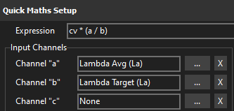
VE Table Quick Validate
a= Lambda Avgb= Lambda Target
This is equivalent to the operation performed when pressing the L key during live tuning. The advantage here is that the the expression can be performed using the the current log cursor position values as inputs.
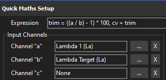
Bank 1 Trim Table Quick Validate
a= Lambda 1*b= Lambda Target*
Similar to the VE expression except that it gives a percentage offset value to be used in the bank trim table. Assumes Bank 1 is measured by Lambda 1.
First the trim is calculated, then the trim is added to the cell value
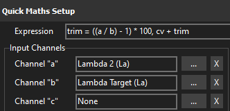
Bank 2 Trim Table Quick Validate
a= Lambda 2b= Lambda Target
Similar to the VE expression except that it gives a percentage offset value to be used in the bank trim table. Assumes Bank 2 is measured by Lambda 2
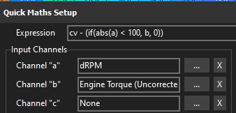
Frictional Loss Table
a= dRPMb= Engine Torque (Uncorrected)
When the engine is accelerating, torque is positive. When the engine is decelerating torque is negative. When the the engine speed is stable (unloaded free revving) the torque is 0. The frictional loss table is used to account for the internal drag of the engine rotating assembly in order to give the correct 0mn final torque value.
The expression checks the dRPM to make sure the engine is held at a near constant RPM (less than a generous 100 rpm/s in this example) where final torque should be 0nm. The abs() function is used to turn a negate dRPM value into a positive to simplify the < (less than) logic. If the dRPM check is true, the current Engine torque value is subtracted from the cell value, if not 0 is subtracted from the cell value, ie. nothing happens.
Calculated Channels
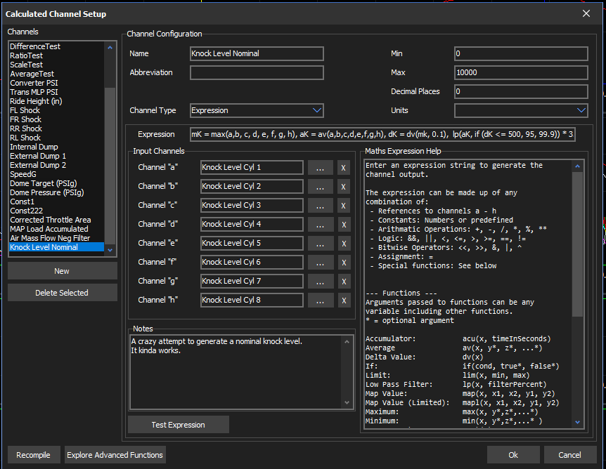
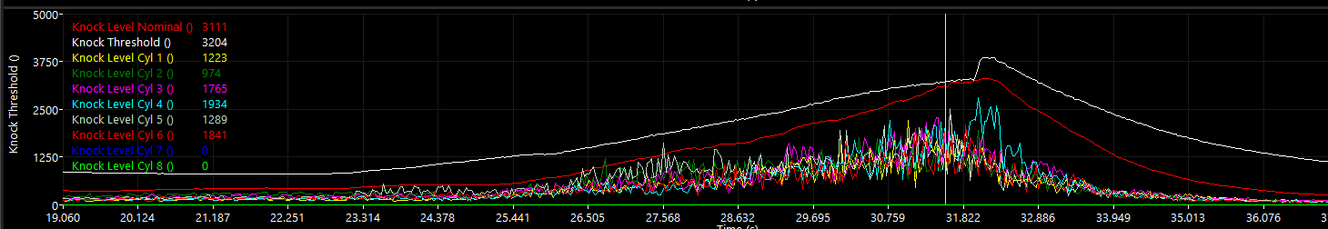
Extreme Example: Knock Threshold Level Helper
a-h= Knk Level Cyl #
An example of using some nested expressions to generate a bit of an idea of what the ideal knock threshold value might be.
The expression finds the max knock (mK), then the average knock (aK), then the derivative of the max over 100ms. Next applies a low pass filter over the average, and adjusts the filter level depending on the derivative. Finally it multiplies the result by 3.2.
This is an example only and isn’t intended to be useful as is for any or all applications. It does however show how functions and variables can be nested in a variety of ways.