Fuel

Fuel Tuning Overview

The fueling calculations used by Emtron are based on an Air Mass per cycle which is then converted to a Fuel Mass based on the requested lambda target. This is true whether the system is using directly measuring airflow from the air mass meter, or calculated air mass from the Ideal Gas Law based on Engine Displacement, Engine Manifold Pressure, Charge Temperature, and Volumetric Efficiency.

Example.

With an engine operating at 85% VE and has a known Charge Temperature and Manifold Pressure, the ECUs calculates an Air Mass per Induction of 0.789 grams. 

To achieve at Lambda target of 0.85 (12.50 AFR petrol) the corresponding fuel mass needs to be 0.06312 grams.

With a known Injector Size in cc/min and Fuel Density (g/ml) the injector mass flow can be determined. Lets use 10.73 grams/sec. 

NOTE: Other factors also affect the injector mass flow. When enabled the ECU monitors the differential pressure across the injector and corrects if it moves away from the nominal static pressure. It does this using “Bernoulli’s equation”  which is a square root law.

Knowing that our fuel injector has a static flow rate of 10.73 grams per second, we divide that into our fuel mass and arrive at a injector pulsewidth value of  5.704 ms

However, the injector cannot just be opened for this time to achieve the calculated Fuel Mass. The Dynamic Characteristics of the fuel injector must be used. This includes injector deadtime and low pulse width non-linearities. 

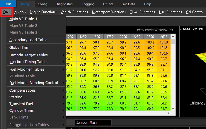
The Graph below of Theoretical vs Actual flow explains this better. The Blue line is the Raw/Theoretical Flow and the Red line is the actual Injector Flow .. note the large error. At 5.7ms the actual fuel mass produced by the injector is 0.0587g instead of the calculated 0.06312 g. 

This is only 93% of the fuel requested.

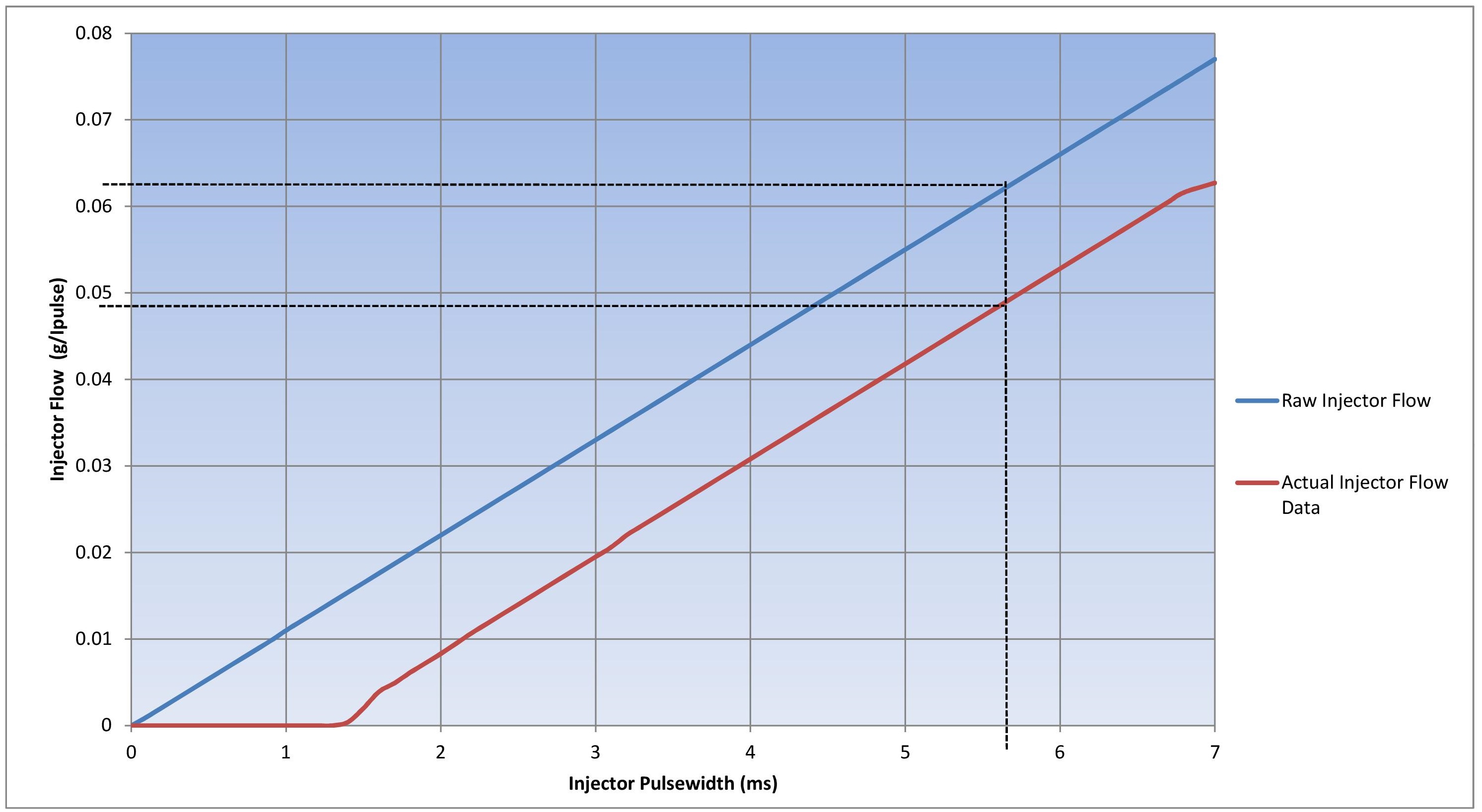
The flow error is caused by an offset that exists between the actual injector flow (Red line) and the theoretical flow (Blue line). This offset exists on all injectors and must be included for the fuel calculation to be accurate.  As the offset is constant across the “majority” of the injector operating range, we can correct for it by adding it to our final injector pulsewidth. This offset error/flow error is known as Injector Deadtime. The ECUs uses a 3D deadtime table spanned on Battery Voltage and Differential Fuel Pressure. See section Injector Deadtime Table for more information.

Once the offset is corrected the Theoretical vs Actual flow graph looks like:

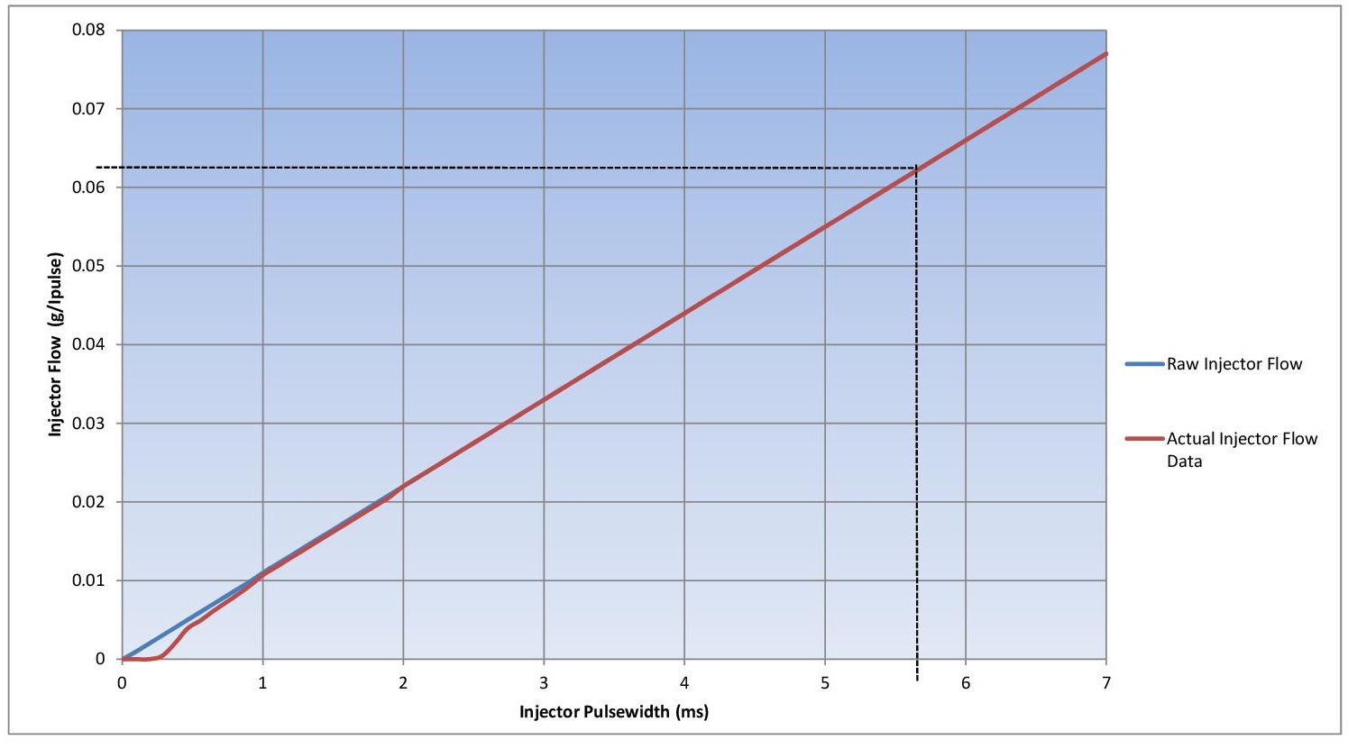
The correction across “most” of the operating range is complete and we can expect the ECU calculated pulsewidth to deliver the requested mass flow. However the range at low pulsewidth still has errors i.e there is a difference between the theoretical and actual pulse with. This is known as the “non linear operating range” of the injector and the graph below has this area zoomed in.

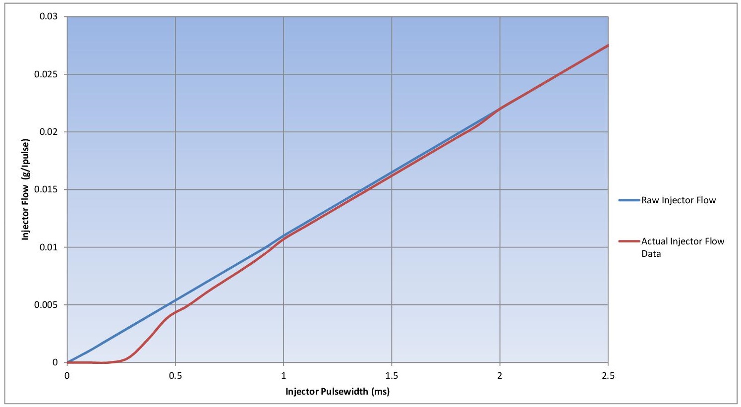
Below 2 ms we have a situation similar to our initial conditions where there was an offset between the actual flow, and theoretical flow of the injector. Unlike the offset within the linear operating range of the injector, this is not constant, and cannot be corrected for with a single value.

The solution is the low pulse adder table which uses offset values that vary with pulsewidth, correcting the lower non linear operating range of the injector. More information can be found Injector Low Pulsewidth Linearisation

With the addition of these values the ECU can achieve nearly perfect fueling down to practically zero flow, and the ECU can do its job of calculating and commanding the correct air fuel ratio under all operating conditions.